HETG simulation of an extended source
The purpose of this example, contributed by Dan Dewey, is to show how to use marx to simulate an HETG observation of a point and a simple extended source with a user-specified spectrum. This example, like many of the other examples, uses marx, Sherpa, and CIAO, which should be installed on your system to run this example.
Create the spectral file
Use MARX to simulate an HETG observation of a powerlaw with two added lines (for example, this could be Fe and Ne fluorescence lines). We will use Sherpa to create a file with model fluxes. This is similar to Simulating a user-defined CCD spectrum with ACIS except that the source is brighter and has a less steep powerlaw.
import numpy as np
from sherpa.astro import ui

# set source properties
ui.set_source(ui.xsphabs.a * ui.xspowerlaw.p + ui.xsgaussian.l1 + ui.xsgaussian.l2)
a.nH = 0.8
p.PhoIndex = 1.2
p.norm = 0.02
l1.lineE = 6.4038  # keV
l2.lineE = 0.8486  # keV
# Make the lines have small but non-zero widths
l1.sigma = 0.05  # about 2300 km/s
l2.sigma = 0.005  # about 1800 km/s
l1.norm = 0.5e-4
l2.norm = 1e-4

# get source
my_src = ui.get_source()

# set energy grid
bin_width = 0.01
energies = np.arange(0.03, 12., bin_width)

# evaluate source on energy grid with lower and upper bin edges
flux = my_src(energies, energies + bin_width)

# MARX input files only have one energy column, and the convention is that
# this holds the UPPER edge of the bin.
# Also, we need to divide the flux by the bin width to obtain the flux density.
ui.save_arrays("source_flux.tbl", [energies + bin_width, flux / bin_width],
               ["keV","photons/s/cm**2/keV"], ascii=True, clobber=True)
Here a fine binning is used having bins with dE/E = 0.0003 (v_bin = 90 km/s). This gives a high resolution spectrum across the whole 1 to 40 Å (0.31 to 12.4 keV) range suitable for use with the HETG as well as, e.g., future microcalorimeter instruments.
The file source_flux.tbl can now be used by marx to define the spectrum.
Setup and run marx
Roughly, these steps are the same as for the previous examples, except that
the HETG is inserted by using GratingType="HETG".
It can be convenient to use pset to set the parameters in a
local par file, but in this case we put together a Python dictionary with options
that we will reformat to match the marx calling. Of course, marx can also be
called directly from the command line, but executing everything from Python
makes it easier for us to re-run these examples and keep everything up to date.
Depending on your problem, it might also be a convenient way for you to script
your marx simulations.
Either way, the first simulation here is for a POINT Source; it is followed by a few additional lines to do a second simulation with a DISK Source.
In the working directory paste these sets of lines to the Python prompt to run a first simulation using a point source:
import subprocess

marxpars = {
    # set the spectrum file to use:
    "SourceFlux": -1,
    "SpectrumType": "FILE",
    "SpectrumFile": "source_flux.tbl",

    # Set other parameters of the simulation:
    # Using 50 ks
    "ExposureTime": 50000,
    "OutputDir": "hetg_plaw",
    "DitherModel": "INTERNAL",

    # Use the HETG with ACIS-S:
    "GratingType": "HETG",
    "DetectorType": "ACIS-S",

    # Some other parameters it can be useful to set:

    # Date of observation (effects ACIS QE)
    "TStart": 2009.5,

    # Roll of the observation: 0 puts average dispersion along E -- W.
    "Roll_Nom": 50,

    # Pointing RA/DEC and source position (degrees)
    "RA_Nom": 250.000,
    "Dec_Nom": -54.000,
    "SourceRA": 250.000,
    "SourceDEC": -54.000,
}

marx_cmd = 'marx ' + ' '.join([f'{k}={v}' for k, v in marxpars.items()])
out = subprocess.call(marx_cmd, shell=True)
# The variable "out" catches the return code here. A value of 0 means success.
assert out == 0
marx runs, ending with something similar to (since marx is a Monte-Carlo based simulation, the exact number of detected photons can vary):
Writing output to directory 'hetg_plaw' ...
Total photons: 3463396, Total Photons detected: 238501, (efficiency: 0.068863)
(efficiency this iteration  0.067985)  Total time: 50000.002238
Now, do another simulation keeping most things the same as above but changing a few things to use a DISK Source:
marxpars["OutputDir"] = "hetg_pldisk"

# Change the SourceType:
marxpars["SourceType"] = "DISK"
# a thin disk with average radius ~ 2.0"
marxpars["S-DiskTheta0"] = 1.7
marxpars["S-DiskTheta1"] = 2.3

marx_cmd = 'marx ' + ' '.join([f'{k}={v}' for k, v in marxpars.items()])
out = subprocess.call(marx_cmd, shell=True)
# The variable "out" catches the return code here. A value of 0 means success.
assert out == 0
Next, we create the fits event file and the aspect solution files for both simulations:
for name in ["plaw", "pldisk"]:
    out = subprocess.call(f'marx2fits hetg_{name} hetg_{name}_evt2.fits', shell=True)
    out = subprocess.call(f'marxasp MarxDir="hetg_{name}" OutputFile="hetg_{name}_asol1.fits"', shell=True)
Note
Combining marx simulations
The tool marxcat allows simulations to be combined, e.g., we
could do the following to make a combination of the point and disk events:
marxcat hetg_plaw hetg_pldisk hetg_plboth
and then create fits and asol files as above. This allows more complex spatial-spectral simulations to be done with marx.
We can look at the simulation output event files with ds9 to check that they are as expected before continuing with ciao-processing. A suitable ds9 command that shows both event files side-by-side and sets up some useful display options is:
ds9 -log -cmap heat hetg_plaw_evt2.fits -regions hetg_plaw_reg1a.fits \
    -scale mode 99.9 hetg_pldisk_evt2.fits -regions hetg_pldisk_reg1a.fits \
    -tile row -saveimage $@ -exit
Alternatively, we can use a small Python script to create similar plots. Here we use
astropy.visualization to do a logarithmic scaling of the images and we use
crates for reading the fits files (crates is part of the CIAO installation):
import pycrates
from astropy.visualization import PercentileInterval, LogStretch, ImageNormalize

fig, axes = plt.subplots(1, 2, figsize=(10,6), subplot_kw={'aspect':'equal'},
                        sharex=True, sharey=True)
bins = [400, 400]
bin_size = 2
range = [[4096 - 0.5 * bin_size * bins[0], 4096 + 0.5 * bin_size * bins[0]],
        [4096 - 0.5 * bin_size * bins[1], 4096 + 0.5 * bin_size * bins[1]]]
for ax, src, title in zip(axes, ["plaw", "pldisk"], ['POINT source', 'DISK source']):
    evt = pycrates.read_file(f'hetg_{src}_evt2.fits')
    hist, x, y = np.histogram2d(evt.get_column('X').values, evt.get_column('Y').values,
                                bins=bins, range=range)
    norm = ImageNormalize(hist, interval=PercentileInterval(99.9), stretch=LogStretch())
    ax.imshow(hist.T, origin='lower', norm=norm, cmap='hot',
            extent=np.array(range).flatten())
    out = ax.set_title(src)
    ax.set_axis_off()

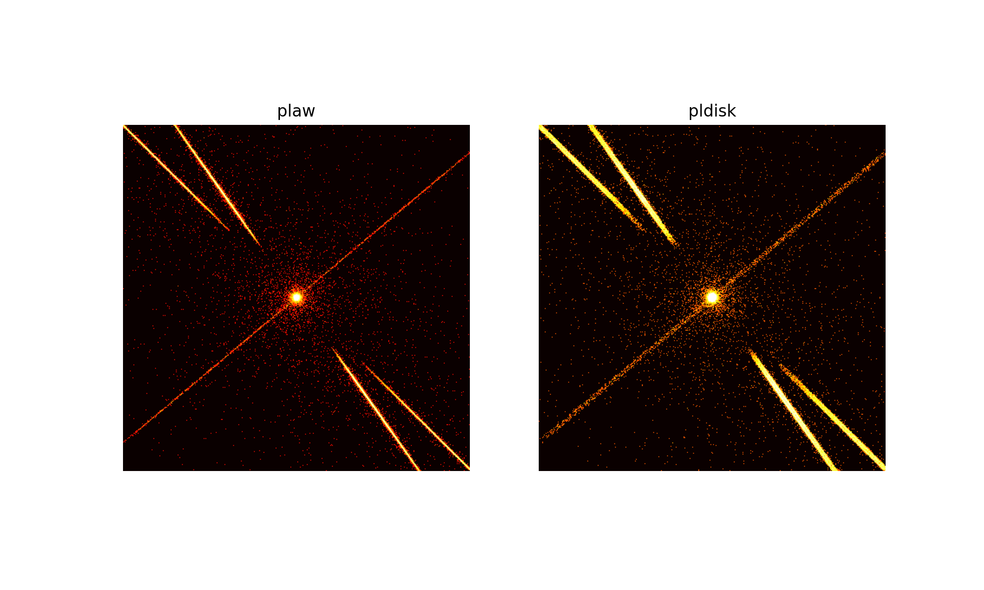
The simulation of the point source is shown on the left, the extended source on the right. The extended source has a much wider zeroth order. Above and below the zeroth order the read-out streak is visible. In both images the X-shape of the grating spectra can be seen. The spectra are much wider in the right image due to the source extension. Still, the grating extraction area that we will calculate below is large enough to capture most of the signal.
We can also use ds9 to record the center of the disk (simulation 2) in X,Y coordinates (4096.5, 4096.5) for further processing.
Extract HETG spectra
We will extract the HETG spectra and then calculate the response matrix for the positive and negative first order in the MEG grating. There is very little signal in the higher orders, so they would not help to constrain the fit significantly. Extraction of the HEG grating works in a similar way, see the CIAO documentation for details.
import ciao_contrib.runtool as rt

# marx2fits generated file
evtfile="hetg_plaw_evt2.fits"

# These files are generated by this script
evt1afile="hetg_plaw_evt1a.fits"
reg1afile="hetg_plaw_reg1a.fits"
asolfile="hetg_plaw_asol1.fits"
pha2file="hetg_plaw_pha2.fits"

rt.tgdetect(infile=evtfile, OBI_srclist_file="NONE", outfile="hetg_plaw_src1a.fits", clobber=True)

rt.tg_create_mask(infile=evtfile, outfile=reg1afile, input_pos_tab="hetg_plaw_src1a.fits",
                grating_obs="header_value", clobber=True, verbose=0)

rt.tg_resolve_events(infile=evtfile, outfile=evt1afile,
                    regionfile=reg1afile, osipfile="CALDB", acaofffile=asolfile,
                    verbose=0, clobber=True)

rt.tgextract(infile=evt1afile, outfile=pha2file, tg_order_list="-1,+1",
            ancrfile="none", respfile="NONE", inregion_file="none", clobber=True,
            tg_srcid_list=1, outfile_type="pha_typeII", tg_part_list='header_value')

for pharow, order in [(3, -1), (4, +1)]:
    rt.mkgrmf(grating_arm="MEG", order=order, outfile=f"meg{order}_rmf.fits", srcid=1,
        detsubsys="ACIS-S3", threshold=1e-06, obsfile=pha2file, regionfile=pha2file,
        wvgrid_arf="compute", wvgrid_chan="compute", clobber=True)

    # fullgarf produces a lot of output. Let's capture that in a variable in case we need it.
    out = rt.fullgarf(phafile=pha2file, pharow=pharow, evtfile=evtfile,
            asol=asolfile, engrid=f"grid(meg{order}_rmf.fits[cols ENERG_LO,ENERG_HI])",
            maskfile="NONE", dafile="NONE", dtffile="NONE", badpix="NONE",
            rootname="", clobber=True,
            # Because marx does not simulate the QE maps, we set ardlibqual=UNIFORM here
            # Because marx does not simulate bad pixels, we set bpmask=0 here
            ardlibqual=";UNIFORM;bpmask=0")
Perform spectral analysis
As an example of spectral analysis, we will fit an absorbed powerlaw to the point-like source spectrum. The spectral regions where the extra lines are located are ignored in the fit. Fitting the spectrum of the extended source works in the similar way. Naturally, a lot more analysis could be done on the simulated spectra, the most obvious point might be a fit of the spectral lines to determine the spectral resolution of Chandra in this example. (The lines from the extended source will appear much wider.) However, that is beyond the scope of this example. Please check the manual of your preferred X-ray spectral fitting software. In this example below, we use Sherpa, but XSPEC and ISIS work very similar.
This is Sherpa code to fit an absorbed powerlaw to the simulated spectrum:
from sherpa.astro import ui
import matplotlib.pyplot as plt
import matplotlib as mpl
from matplotlib import ticker

ui.load_pha(pha2file)
ui.load_arf(3, 'MEG_-1_garf.fits')
ui.load_rmf(3, 'meg-1_rmf.fits')
ui.load_arf(4, 'MEG_1_garf.fits')
ui.load_rmf(4, 'meg1_rmf.fits')
ui.set_source(3, ui.xsphabs.a * ui.xspowerlaw.xp)
ui.set_source(4, ui.xsphabs.a * ui.xspowerlaw.xp)
# We didn't make ARF and RMF for the HEG, so we can't do anything
# in energy space there. So, we loop to apply setting only to the MEG arms.
for i in [3, 4]:
    # ignore the lines in the fit
    ui.set_analysis(i, "energy")
    ui.ignore_id(i, None, 0.5)
    ui.ignore_id(i, 0.8, 0.9)
    ui.ignore_id(i, 6.3, 6.5)
    ui.ignore_id(i, 8.0, None)
    ui.group_counts(i, 25)
ui.fit(3, 4)

# Now, plot the fit
ui.plot_data(3, yerrorbars=False, color='C0', alpha=0.4, xlog=True, ylog=False, markersize=4)
ui.plot_data(4, yerrorbars=False, overplot=True, color='C1', alpha=0.4, markersize=4)
ui.plot_model(3, color='C0', overplot=True, label='MEG -1')
ui.plot_model(4, overplot=True, color="C1", label='MEG +1')
plt.legend()
plt.title("")

# By default, matplotlib labels only 10^0, 10^1 etc. in log plots.
# That would give us only a single xlabel on this plot.
# The following lines change the matplotlib settings for the formatting
# of the x-axis to show more ticks.
ax = plt.gca()
mpl.rcParams['axes.formatter.min_exponent'] = 2
ax.get_xaxis().set_minor_formatter(ticker.LogFormatterMathtext(labelOnlyBase=False,
                                                            minor_thresholds=(2, .5)))
ax.tick_params(axis='x', labelsize=mpl.rcParams['xtick.labelsize'], which='both')

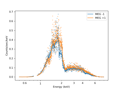
The resulting fit parameters are similar, but not identical, to the parameters we put into the simulation above.
Datapoints are shown slightly transparent and without error bars because the plot would be too messy otherwise. The solid lines show the fitted model. The MEG orders in the plot differ from one another because the effective area is different, e.g. the gaps between the ACIS chips fall on different wavelengths.
