Simulating a thermal plasma with the HETGS grating
The purpose of this example is to show how to use marx to simulate an HETG grating spectrum of a star whose spectrum is represented by an APEC model.
Creating the spectral file for marx
As in Simulating a user-defined CCD spectrum with ACIS, we will use Sherpa again to generate the spectral file from the parameter file describing the model. The procedure to define the model is very similar to the one used in Simulating a user-defined CCD spectrum with ACIS, except that we will use a much finer energy grid for the model. Here is a model with two thermal components. Since we don’t define an interstellar absorption for this example, there is a lot of flux at low energies.
from sherpa.astro import ui

# set source properties
ui.set_source(ui.xsvapec.a1 + ui.xsvapec.a2)
a1.norm, a2.norm = 0.016, 0.0156
a1.kT, a2.kT = 8.5, 2.8  # in keV
a2.Ne = a1.Ne
a2.Fe = a1.Fe
a1.Ne = 2
a1.Fe = 0.2

my_src = ui.get_source()
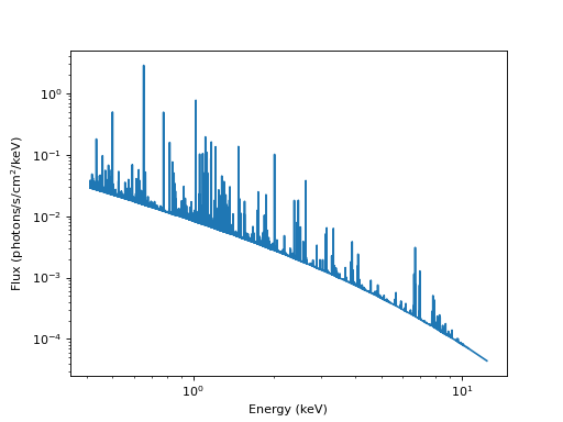
Like in the previous example, we will arrange bins (this time in wavelength space) and write the tabulated model to a file. We will use a grid from 1 to 30 Angstrom with 16384 bins.
import numpy as np
from matplotlib import pyplot as plt

# set energy grid
wavelength = np.linspace(1., 30., 16384)  # in Angstrom
# convert to keV
energies = 12.39842 / wavelength  # keV
# for simplicity, reverse to have array ascending in energy
energies = energies[::-1]

# evaluate source on energy grid with lower and upper bin edges
flux = my_src(energies[:-1], energies[1:])

# MARX input files only have one energy column, and the convention is that
# this holds the UPPER edge of the bin.
# Also, we need to divide the flux by the bin width to obtain the flux density.
bin_width = energies[1:] - energies[:-1]
ui.save_arrays("apedflux.tbl", [energies[1:], flux / bin_width],
            ["keV","photons/s/cm**2/keV"], ascii=True, clobber=True)

midbin = 0.5 * (energies[:-1] + energies[1:])
plt.loglog(midbin, flux / bin_width)
plt.xlabel("Energy (keV)")
plt.ylabel("Flux (photons/s/cm$^2$/keV)")
Running marx for the HETGS
The next step is to run marx in the desired configuration. For this
example, ACIS-S and the HETG are used. Here, we will wrap the marx call
into a Python script. Since marx currently does not have a “nice” Python
interface, we run it via subprocess.call():
import subprocess
out = subprocess.call('marx SourceFlux=-1 SpectrumType="FILE" ' + \
         'SpectrumFile="apedflux.tbl" ExposureTime=80000 OutputDir=aped ' +\
         'DitherModel="INTERNAL" ' +\
         'GratingType="HETG" DetectorType="ACIS-S"', shell=True)
This will run the simulation and place the results in a subdirectory
called aped. The results may be converted to a standard Chandra
level-2 fits file by the marx2fits program:
evtfile="aped_evt2.fits"
out = subprocess.call(f'marx2fits aped {evtfile}', shell=True)
The resulting fits file aped_evt2.fits may be further processed
with standard CIAO tools, as described below. As some of these tools
require the aspect history, the marxasp program will be used to
create an aspect solution file that matches the simulation:
asol1file="aped_asol1.fits"
out = subprocess.call(f'marxasp MarxDir="aped" OutputFile="{asol1file}"', shell=True)
Creating a type-II PHA file
For a Chandra grating observation, the CIAO tgextract tool may used to create a type-II PHA file. Before this can be done, an extraction region mask file must be created using tg_create_mask, followed by order resolution using tg_resolve_events. The first step is to determine the source position, which is used by tg_create_mask. There are many ways to do this; the easiest might be to open the event file in ds9, put a circle on the source position and use the ds9 functions to center it. In this example use the find zero-order algorithm of findzo , which is robust enough to work on heavily piled-up sources with read-out streaks, which is implemented in tgdetect.
We are using a Python interface to CIAO to run the CIAO tools to
create a PHA2 file called aped_pha2.fits:
import ciao_contrib.runtool as rt

evt1afile = "aped_evt1a.fits"
reg1afile = "aped_reg1a.fits"
pha2file = "aped_pha2.fits"
srcfile = "src1a.fits"
asol1file="aped_asol1.fits"

rt.tgdetect(infile=evtfile, outfile="letgplaw_src1a.fits", clobber=True)

rt.tg_create_mask(infile=evtfile, outfile=reg1afile, input_pos_tab="letgplaw_src1a.fits",
                clobber=True)

rt.tg_resolve_events(infile=evtfile, outfile=evt1afile, regionfile=reg1afile,
                    acaofffile=asol1file, clobber=True)

rt.tgextract(infile=evt1afile, outfile=pha2file, tg_order_list="-1,+1", tg_srcid_list=1,
            clobber=True)
An important by-product of this script is the evt1a file, which
includes columns for the computed values of the wavelengths and orders
of the diffracted events. In fact, tgextract makes use of
those columns to create the PHA2.
As usual, we again want to generate the response files. With the setting above,
the PHA2 file contains four spectra, MEG and HEG, each with positive and negative
orders. Here, we will create the RMF and ARF for the MEG +1 order only. Note that
we set the ardlibqual=";UNIFORM;bpmask=0" for the fullgarf call
to get a uniform ARF without any bad pixel masking and assuming a uniform quantum
efficiency across the detector because those are the assumptions that marx makes
in the simulation.
rt.mkgrmf(grating_arm="MEG", order=1, outfile="meg1.rmf", srcid=1, detsubsys="ACIS-S3", obsfile=evtfile,
          regionfile=pha2file, clobber=True)
rt.fullgarf(phafile=pha2file, pharow=4, evtfile=evtfile, asol=asol1file, engrid="grid(meg1.rmf[cols ENERG_LO,ENERG_HI])",
            ardlibqual=";UNIFORM;bpmask=0", clobber=True, verbose=0)
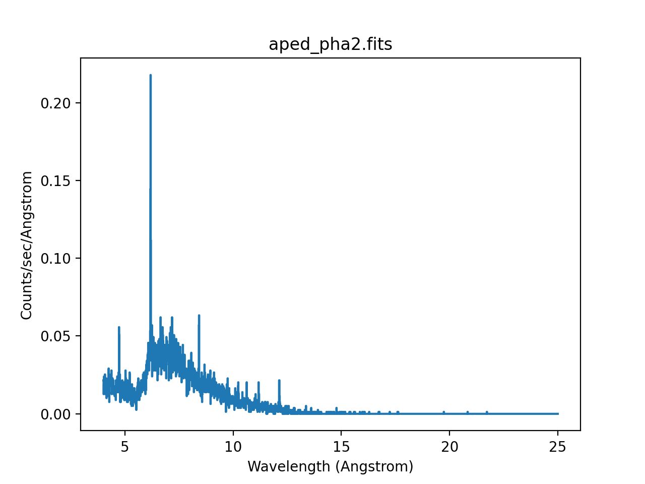
The resulting event file may be loaded into Sherpa. Since the PHA2 file contains four spectra, Sherpa creates for datasets, labelled 1 to 4. The last one is the MEG +1 spectrum, which we will plot here:
ui.load_pha(pha2file)
ui.load_rmf(4, "meg1.rmf")
ui.load_arf(4, "MEG_1_garf.fits")
ui.set_analysis(4, "wave")
ui.group_width(4, 2)
ui.notice_id(4, 4., 25.)
ui.plot_data(4, yerrorbars=False, linestyle='solid', marker=None)
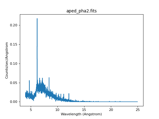
Here, we used group_width() to group neighboring bins together.
