Simulating a user-defined CCD spectrum with ACIS¶

The purpose of this example is to show how to use marx to simulate an ACIS observation of a point source with a user-specified spectrum. For simplicity, suppose that we wish to simulate a 3000 ksec observation of an on-axis point source whose spectrum is represented by an absorbed powerlaw, with a spectral index of 1.8, and a column density of $10^{22}$ atoms/cm^2. The normalization of the powerlaw will be set to 0.001 photons/keV/cm^2/s at 1 keV. The large exposure time was chosen to illustrate the consistency of the marx ray trace with that of the underlying calibration data.

Creating the spectral file¶

The first step is to create a 2-column text file that tabulates the flux [photons/sec/keV/cm^2] (second column) as a function of energy [keV] (first column). The easiest way to create such a file is to make use of a spectral modeling program such as ISIS, Sherpa or XSpec. The rest of this tutorial is given in the context of Sherpa.

In Sherpa the absorbed powerlaw model is specified using:

from sherpa.astro import ui

# set source properties
ui.set_source(ui.xsphabs.a * ui.xspowerlaw.p)
a.nH = 1.
p.PhoIndex = 1.8
p.norm = 0.001

my_src = ui.get_source()
print(str(my_src))

The model parameters lists by Sherpa should look like this:

xsphabs.a * xspowerlaw.p
   Param        Type          Value          Min          Max      Units
   -----        ----          -----          ---          ---      -----
   a.nH         thawed            1            0        1e+06 10^22 atoms / cm^2
   p.PhoIndex   thawed          1.8           -3           10
   p.norm       thawed        0.001            0        1e+24

The next step is to convert the parameter file plaw.p to the spectrum file that marx expects. We can use the commands below (see also the Sherpa thread http://cxc.harvard.edu/sherpa/threads/marx/ for another example):

import numpy as np
# set energy grid
bin_width = 0.003
energies = np.arange(0.03, 12., bin_width)

# evaluate source on energy grid with lower and upper bin edges
flux = my_src(energies, energies + bin_width)

# MARX input files only have one energy column, and the conventions is that
# this hold the UPPER edge of the bin.
# Also, we need to divide the flux by the bin width to obtain the flux density.
ui.save_arrays("plawflux.tbl", [energies + bin_width, flux / bin_width],
            ["keV","photons/s/cm**2/keV"], ascii=True, clobber=True)

ISIS users can make use of the marxflux script and for XSpec users, marx is distributed with a script called xspec2marx that may be used to create such a file.

The plawflux.tbl file is input to marx using the following marx.par parameters:

SpectrumType=FILE
SpectrumFile=plawflux.tbl
SourceFlux=-1

The SpectrumType parameter is set to FILE to indicate that marx is to read the spectrum from the file specified by the SpectrumFile parameter. The SourceFlux parameter may be used to indicate the integrated flux of the spectrum. The value of -1 as given above means that the integrated flux is to be taken from the file.

Running marx for this powerlaw spectrum¶

The next step is to run marx in the desired configuration. Some prefer to use tools such as pset to update the marx.par file and then run marx or to pass the arguments via the command line in a shell. Here, we will wrap the marx call into a Python script. Since marx currently does not have a “nice” Python interface, we run it via subprocess.call():

import subprocess

out = subprocess.call('marx SourceFlux=-1 SpectrumType="FILE" SpectrumFile="plawflux.tbl" ' + \
'ExposureTime=100000 TStart=2012.5 ' + \
'OutputDir=plaw GratingType="NONE" DetectorType="ACIS-S" ' + \
'DitherModel="INTERNAL" RA_Nom=30 Dec_Nom=40 Roll_Nom=50 ' + \
'SourceRA=30 SourceDEC=40 ', shell=True)

This will run the simulation and place the results in a subdirectory called plaw. The results may be converted to a standard Chandra level-2 fits file by the marx2fits program:

subprocess.call("marx2fits plaw plaw_evt2.fits", shell=True)

The resulting fits file plaw_evt2.fits may be further processed with standard CIAO tools. As some of these tools require the aspect history, the marxasp program will be used to create an aspect solution file that matches the simulation:

subprocess.call("marxasp MarxDir='plaw' OutputFile='plaw_asol1.fits'", shell=True)

Creating CIAO-based ARFs and RMFs for MARX Simulations¶

Armed with the simulated event file plaw_evt2.fits and the aspect solution file plaw_asol1.fits, a PHA file, ARF and RMF may be made using the standard CIAO tools. First, extract the PHA data. The asphist CIAO tool may be used to create an aspect histogram from an aspect solution file. Again, we are using a Python interface to CIAO to run the CIAO tools:

from ciao_contrib import runtool as rt
# Extraction region parameters: circle of radius R at (X,Y)
X=4096.5
Y=4096.5
R=20.0

phagrid="pi=1:1024:1"

evtfile="plaw_evt2.fits"
asolfile="plaw_asol1.fits"
phafile="plaw_pha.fits"
rmffile="plaw_rmf.fits"
arffile="plaw_arf.fits"
asphistfile="plaw_asp.fits"

rt.asphist(infile=asolfile, outfile=asphistfile, evtfile=evtfile, clobber=True)

rt.dmextract(infile=f"{evtfile}[sky=Circle({X},{Y},{R})][bin {phagrid}]",
outfile=phafile, clobber=True)

While marx strives to accurately model of the Chandra Observatory, there are some differences that need to be taken into account when processing marx generated data with CIAO. As described in Current caveats for MARX page, marx does not incorporate the non-uniformity maps for the ACIS detector, nor does it employ the spatially varying CTI-corrected pha redistribution matrices (RMFs). As such there will be systematic differences between the marx ACIS effective area and that of the mkarf CIAO tool when run in its default mode. Similarly, the mapping from energy to pha by marx will be different from that predicted by mkacisrmf.

Creating an ARF to match a marx simulation¶

As mentioned above, marx does not implement the ACIS QE uniformity maps. The following commands show how to set the mkarf parameters to produce an ARF that is consistent with the marx effective area (this continues the Python script from the last paragraph):

# Select a CCD.
ccdid=7

detname=f"ACIS-{ccdid};UNIFORM;bpmask=0"
# For ACIS-I, use engrid="0.3:11.0:0.003". This reflects a limitation of mkrmf.
engrid="0.3:12.0:0.003"

rt.mkarf.punlearn()
rt.mkarf(detsubsys=detname, outfile=arffile, obsfile=evtfile, engrid=engrid,
         asphistfile=asphistfile, sourcepixelx=X, sourcepixely=Y, clobber=True)

Notice the settings detsubsys="ACIS-7;uniform;bpmask=0" and maskfile=NONE pbkfile=NONE dafile=NONE that are different from the way a normal Chandra observation would be processed.

Creating an RMF to match a marx simulation¶

marx maps energies to phas using the FEF gaussian parametrization utilized by the mkrmf CIAO tool. The newer mkacisrmf tool uses a more complicated convolution model that does not appear to permit a fast, memory-efficient random number generation algorithm that marx would require. In contrast, a gaussian-distributed random number generator is all that is required to produce pha values that are consistent with mkrmf generated responses.

The Chandra CALDB includes several FEF files. The one that marx currently employs is acisD2000-01-29fef_phaN0005.fits, and is located in the $CALDB/data/chandra/acis/cpf/fefs/ directory. This file must be specified as the infile mkrmf parameter.

For a point source simulation, look at the marx2fits generated event file and find the average chip coordinates. The CIAO dmstat tool may be used for this purpose. The CCD_ID and the mean chip coordinates are important for the creation of the filter that will be passed to mkrmf to select the appropriate FEF tile. For simplicity suppose that the mean point source detector location is at (308,494) on ACIS-7. Then run mkrmf using (continuing the shell script form above):

import os
# Mean chip position
chipx=221
chipy=532

fef=f"{os.environ['CALDB']}/data/chandra/acis/fef_pha/acisD2000-01-29fef_phaN0005.fits"

cxfilter=f"chipx_hi>={chipx},chipx_lo<={chipx}"
cyfilter=f"chipy_hi>={chipy},chipy_lo<={chipy}"
rt.mkrmf(infile=f"{fef}[ccd_id={ccdid},{cxfilter},{cyfilter}]", outfile=rmffile,
         axis1=f"energy={engrid}", axis2=phagrid, clobber=True)

Notice, how the FEF file is set explicitly to fef="$CALDB/data/chandra/acis/cpf/fefs/acisD2000-01-29fef_phaN0005.fits" (where we use Python to retrieve the $CALDB environment variable) and that the correct tile of that FEF file is chosen with fef[ccd_id=7,chipx_hi>=221,chipx_lo<=221,chipy_hi>=532,chipy_lo<=532]

See the CIAO threads for other ways of running mkrmf. The important thing is to specify the correct FEF and tile.

Analyzing the simulated data¶

The PHA, ARF, and RMF files may be used in a spectral modelling program such as Sherpa to see whether or not one can reach the desired science goal from the simulated observation. For this example, the goal is to verify that the marx simulation is consistent with the input spectrum. To this end, Sherpa will be used to fit an absorbed powerlaw to the pha spectrum. The figure below showing the resulting fit was created via the following script:

ui.load_pha(phafile)
ui.load_rmf(rmffile)
ui.load_arf(arffile)
ui.group_counts(25)
ui.set_source(ui.xsphabs.a * ui.xspowerlaw.p)
a.nH = 0.001
p.PhoIndex = 1.8
p.norm = 0.1
ui.ignore(None, 0.4)
ui.ignore(10.0, None)
ui.fit()

This script produced the following parameter values with a an acceptable reduced chi-square (“rstat”, the reduced value of the statistic, which in this case is a variant of the chi-square statistic):

datasets       = (1,)
itermethodname = none
methodname     = levmar
statname       = chi2gehrels
succeeded      = True
parnames       = ('a.nH', 'p.PhoIndex', 'p.norm')
parvals        = (1.0056518439746143, 1.8249105691365235, 0.0009957222213215742)
statval        = 250.83362547852525
istatval       = 8228197308.198434
dstatval       = 8228197057.364808
numpoints      = 354
dof            = 351
qval           = 0.99998601702262
rstat          = 0.714625713614032
message        = successful termination
nfev           = 78

The rplot_counts may be used to produce a plot of the resulting fit.

import matplotlib.pyplot as plt

ui.plot_fit_delchi(xlog=True, ylog=True)
plt.gcf().axes[0].set_title("Simulated spectrum and fit without pile-up")

(png, hires.png, pdf)

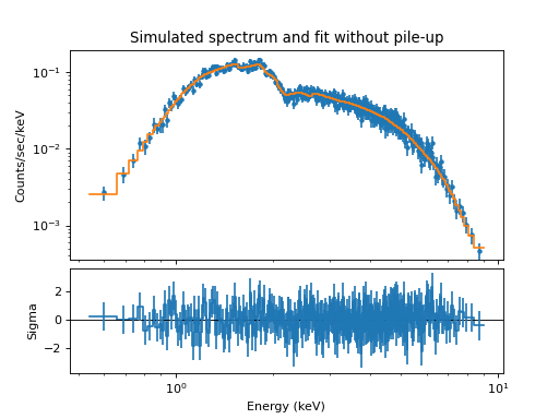
The residuals show that the model is systematically high for some energies. The reason for this can be traced back to energy-dependent scattering where photons are scattered outside the extraction region. The CIAO effective area does not include this loss factor, and as a result, this omission appears in the residuals. This effect is apparant because of the enormous number of counts in this simulation.

Simulating pile-up in an ACIS CCD spectrum¶

The purpose of this example is to show how to to use the marxpileup program to simulate the effects of pileup. Pileup occurs when two or more photons land in the same pixel location in a given ACIS readout time. marxpileup is a post-processor that performs a frame-by-frame analysis of an existing marx simulation. We continue the example from above, where the spectrum had a somewhat large normalization to ensure that pileup would occur.

Creating an event file with pile-up¶

marxpileup can be run on the eventfile generated by marx using:

subprocess.call("marxpileup MarxOutputDir=plaw", shell=True)

This will create a directory called plaw/pileup/ and place the pileup results there. It also writes a brief summary to the display resembling:

Total Number Input: 770961
Total Number Detected: 482771
Efficiency: 6.261938e-01

This shows that because of pileup, nearly 40 percent of the events were lost.

The next step is to run marx2fits to create a corresponding level-2 file called plaw_pileup_evt2.fits.

subprocess.call("marx2fits --pileup plaw/pileup plaw_pileup_evt2.fits", shell=True)

Since this is a pileup simulation, the --pileup flag was passed to marx2fits.

In this case we can use the same ARF and RMF as above. However, it is necessary to create a new PHA file from the plaw_pileup_evt2.fits event file. For analyzing a piled observation of a near on-axis point source, it is recommended that the extraction region have a radius of 4 ACIS tangent plane pixels.

# Smaller radius this time
R=4.0

evtfile="plaw_pileup_evt2.fits"
phafile="plaw_pileup_pha.fits"

rt.dmextract(infile=f"{evtfile}[sky=Circle({X},{Y},{R})][bin {phagrid}]",
outfile=phafile, clobber=True)

Analyzing the pile-up simulated data¶

As before, Sherpa will be used to analyze the piled spectrum.

ui.load_pha("pileup", "plaw_pileup_pha.fits")
ui.load_rmf("pileup", rmffile)
ui.load_arf("pileup", arffile)
ui.group_counts("pileup", 25)
ui.set_source("pileup", ui.xsphabs.apileup * ui.xspowerlaw.pileup)
a.nH = 1
p.PhoIndex = 1.8
p.norm = 0.001
ui.ignore(None, 0.4)
ui.ignore(10.0, None)
ui.fit("pileup")

The fit produces the following results:

datasets       = ('pileup',)
itermethodname = none
methodname     = levmar
statname       = chi2gehrels
succeeded      = True
parnames       = ('apileup.nH', 'pileup.PhoIndex', 'pileup.norm')
parvals        = (0.8278883441194863, 1.4482348891214787, 0.0003778956786769391)
statval        = 291.04582161109454
istatval       = 168746129070.67175
dstatval       = 168746128779.62595
numpoints      = 316
dof            = 313
qval           = 0.808410809336432
rstat          = 0.9298588549875225
message        = successful termination
nfev           = 33

Note that the parameters are different from the power-law parameters that went into the simulation. For example, the normalization is less than what was expected, and the powerlaw index is somewhat low compared to the expected value of 1.8.

Suspecting that this observation suffers from pileup, we enable the Sherpa pileup kernel, which introduces a few additional parameters:

ui.set_pileup_model("pileup", ui.jdpileup.jdp)

which gives us the following model:

xsphabs.a * xspowerlaw.p
   Param        Type          Value          Min          Max      Units
   -----        ----          -----          ---          ---      -----
   a.nH         thawed            1            0        1e+06 10^22 atoms / cm^2
   p.PhoIndex   thawed          1.8           -3           10
   p.norm       thawed        0.001            0        1e+24

Given the fact that the PSF fraction varies with off-axis angle and spectral shape, we will allow it to vary during the fit.

As before, the fit command may be used to compute the best fit parameters. However, the parameter space in the context of the pileup kernel can be complex with many local minima, even for a function as simple as an absorbed powerlaw. For this reason it might be useful to start the fit multiple times from different starting points or use an ompimizer such as a Monte-Carlo algorithm to explore the parameter space more fully.:

ui.fit("pileup")

The above produces:

datasets       = ('pileup',)
itermethodname = none
methodname     = levmar
statname       = chi2gehrels
succeeded      = True
parnames       = ('jdp.alpha', 'jdp.f', 'apileup.nH', 'pileup.PhoIndex', 'pileup.norm')
parvals        = (0.204790003483574, 0.9336190568894115, 0.9756775711805925, 1.800359678118324, 0.0012576164479282882)
statval        = 225.68345370560232
istatval       = 1192.623686707686
dstatval       = 966.9402330020836
numpoints      = 316
dof            = 311
qval           = 0.9999178701372992
rstat          = 0.7256702691498467
message        = successful termination
nfev           = 47

We see that the reduced chi-square is near what one would expect for a good fit and that the powerlaw index is very close to the expected value. We can use the ui.conf() function to obtain its confidence interval if we want to.

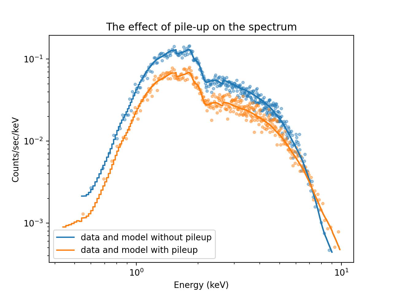
Here is a plot of the resulting fit. We use the Sherpa plotting function ui.plot_data and pass several options to customize the plot. Options that are not processed by Sherpa itself are passed to matplotlib (e.g. color=’C0’ set the first color in the default color cycle in matplotlib).

ui.plot_data(yerrorbars=False, color='C0', alpha=0.4, xlog=True, ylog=True)
ui.plot_data("pileup", yerrorbars=False, overplot=True, color='C1', alpha=0.4)
ui.plot_model(color='C0', overplot=True, label='data and model without pileup')
ui.plot_model("pileup", overplot=True, color="C1", label='data and model with pileup')
plt.legend()
plt.title("The effect of pile-up on the spectrum")