Simulating an LETG/ACIS-S observation
In this example, we simulate an LETG/ACIS-S observation with marx. The primary goal of this exercise is to see how well marx can simulate this instrument combination by performing a spectral analysis of the result. For simplicity, we assume an on-axis point source and an absorbed powerlaw spectrum with a column density of \(10^{19}\) atoms/cm^2, a spectral index of 1.8. Rather than specifying an exposure time for the observation as in the other examples, here we specify the desired number of detected events. In this case, the simulation will be run until 100,000 (1e5) events have been detected.
Creating an input spectrum from a Sherpa model
The first step is to create a 2-column text file that tabulates the absorbed powerlaw flux [photons/sec/keV/cm^2] (second column) as a function of energy [keV] (first column). The easiest way to create such a file is to make use of a spectral modeling program. For a change, we will use the Sherpa program in this example.
We chose the specific physical model (a positive powerlaw with an unrealistically high flux) because we want to construct a really detailed picture of the features seen in the PSF and we need a large number of photons over a wide range of energies:
import numpy as np
from sherpa.astro import ui

# set source properties
ui.set_source(ui.xsphabs.a * ui.xspowerlaw.p)
a.nH = 0.001
p.PhoIndex = 1.8
p.norm = 0.1

# get source
my_src = ui.get_source()

# set energy grid
bin_width = 0.01
energies = np.arange(0.03, 12., bin_width)

# evaluate source on energy grid with lower and upper bin edges
flux = my_src(energies, energies + bin_width)

# MARX input files only have one energy column, and the conventions is that
# this hold the UPPER edge of the bin.
# Also, we need to divide the flux by the bin width to obtain the flux density.
ui.save_arrays("source_flux.tbl", [energies + bin_width, flux / bin_width],
               ["keV","photons/s/cm**2/keV"], ascii=True, clobber=True)
More details about the format of the marx input spectrum can be found at SpectrumFile.
Note, that the parameter SourceFlux sets the normalization of the flux; if the
normalization of the model file should be used, set SourceFlux=-1.
Running marx
The next step is to run marx in the desired configuration. Some
prefer to use tools such as pset to update the marx.par
file and then run marx. Here, the parameters will be explicitly
passed to marx. Currently, marx can only be run from the command line.
So we run it via subprocess.call() in our Python script:
import subprocess
out = subprocess.call('marx SourceFlux=-1 SpectrumType="FILE" SpectrumFile="source_flux.tbl" ' +
    'NumRays=-100000 ExposureTime=0 TStart=2012.5 ' +
    'OutputDir=letgplaw GratingType="LETG" DetectorType="ACIS-S" ' +
    'DitherModel="INTERNAL" RA_Nom=30 Dec_Nom=40 Roll_Nom=50 ' +
    'SourceRA=30 SourceDEC=40 Verbose=0', shell=True)
# The variable "out" catches the return code here. A value of 0 means success.
assert out == 0
Note the use of a negative value of the NumRays parameter.
This tells marx that the simulation is to continue until the absolute
value of that number of rays have been detected.
The SourceFlux parameter may be used to indicate the integrated flux of
the spectrum. The value of -1
as given above means that the integrated flux is to be taken from the file.
The results of the
simulation will be written to a subdirectory called letgplaw, as
specified by the OutputDir parameter. After the simulation has
completed, a standard Chandra event file may be created using the marx2fits
program:
out = subprocess.call('marx2fits letgplaw letgplaw_evt.fits', shell=True)
The fits file letgplaw_evt.fits can be further processed
with standard CIAO tools. As some of these tools require the aspect
history, the marxasp program is used to create an aspect
solution file that matches the simulation:
out = subprocess.call('marxasp MarxDir="letgplaw" OutputFile="letgplaw_asol1.fits"', shell=True)
It is interesting to look at the event file with a viewer such as ds9. Here we use dmimg2jpg, which displays an RGB image of the events projected to the sky plane.
# Can't call with runtool because of https://cxc.cfa.harvard.edu/ciao/ahelp/ciao_runtool.html#Redirected_values
# see https://github.com/cxcsds/ciao-contrib/issues/1015 for discussion
out = subprocess.call('dmimg2jpg "letgplaw_evt.fits[x=3950:4250][y=3950:4250][energy=0:500][bin sky=1]" ' +
             '"letgplaw_evt.fits[x=3950:4250][y=3950:4250][energy=500:2000][bin sky=1]" ' +
             '"letgplaw_evt.fits[x=3950:4250][y=3950:4250][energy=2000:12000][bin sky=1]" ' +
             'regionfile="" outfile="image_rgb.jpg" minred=0 mingreen=0 minblue=0 maxred=10 ' +
             'maxgreen=50 maxblue=50 clobber=yes', shell=True)

import matplotlib.image as mpimg
import matplotlib.pyplot as plt
img = mpimg.imread('image_rgb.jpg')
plt.imshow(img)
plt.axis('off')
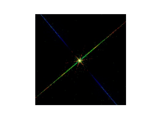
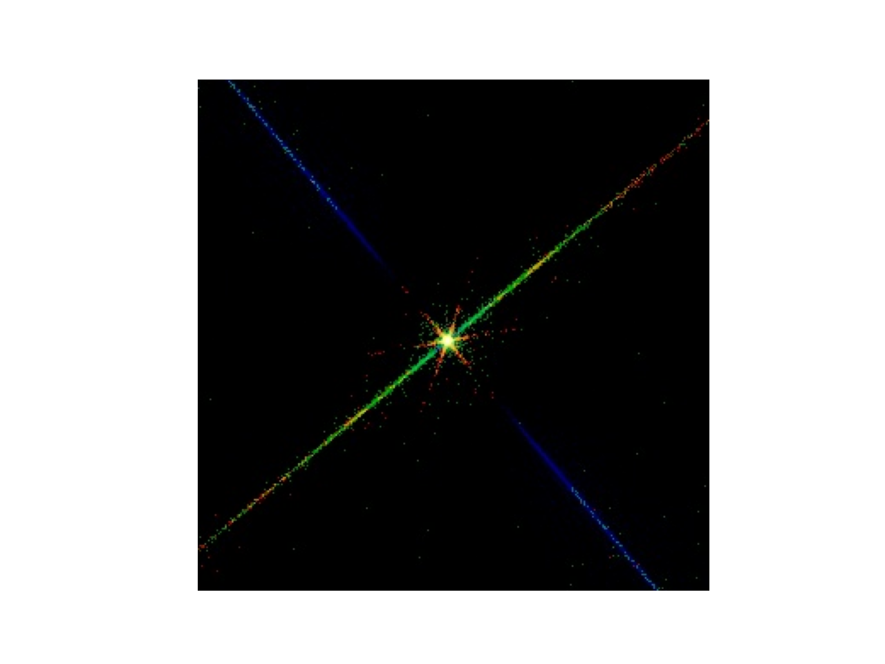
RGB image of the event file. The energy bands were color-coded as follows: red: 0.0 to 0.5 keV, green: 0.5 to 2.0 keV, blue: 2.0 to 12 keV.
This image shows what the pattern of events looks like near zeroth order. There are a number of features in this image that are worth pointing out. The thick blue line in the middle of the fan-like structure that extends from the top left of the figure to the bottom right corresponds to diffracted photons from the primary grating bars of the LEG. The events in this line are the subject of the spatial extraction step when creating the event histograms for spectral analysis, as described below. The other blue lines in the fan-like structure (very faint, comes out better in longer simulations) correspond to photons that have also been diffracted by the fine support structure of the LEG. This fine support structure forms a grating that diffracts in a direction orthogonal to the primary diffraction direction. The events in the multicolored line that runs from the bottom left to the upper right consists of two contributions. The first is from photons that arrived at the detector while the image was being read out between frames. The second is from the undiffracted photons from the primary grating that have been diffracted from the LEG fine support structure. The red star-like pattern in the center of the figure was produced by photons that have diffracted from the LEG’s coarse support structure, whose 2 mm period diffracts only the very lowest energy photons through an appreciable angle. Finally, if one looks closely enough, the shadowing of the mirror support struts may be seen near zeroth order.
Analyzing the data simulated by marx
The (type-II) PHA file, grating ARFs and RMFs can be produced using the
standard CIAO tools using the simulated event file
letgplaw_evt.fits and the aspect solution file
letgplaw_asol1.fits as inputs. Here is a Python script that does
this:
import ciao_contrib.runtool as rt

# marx2fits generated file
evtfile="letgplaw_evt.fits"

# These files are generated by this script
evt1afile="letgplaw_evt1a.fits"
reg1afile="letgplaw_reg1a.fits"
asolfile="letgplaw_asol1.fits"
pha2file="letgplaw_pha2.fits"

rt.tgdetect(infile=evtfile, OBI_srclist_file="NONE", outfile="letgplaw_src1a.fits", clobber=True)

rt.tg_create_mask(infile=evtfile, outfile=reg1afile, input_pos_tab="letgplaw_src1a.fits",
                grating_obs="header_value", clobber=True, verbose=0)

rt.tg_resolve_events(infile=evtfile, outfile=evt1afile,
                    regionfile=reg1afile, osipfile="CALDB", acaofffile=asolfile,
                    verbose=0, clobber=True)

rt.tgextract(infile=evt1afile, outfile=pha2file, tg_order_list="-1,+1",
            ancrfile="none", respfile="NONE", inregion_file="none", clobber=True,
            tg_srcid_list=1, outfile_type="pha_typeII", tg_part_list='header_value')

rt.mkgrmf(grating_arm="LEG", order=-1, outfile="leg-1_rmf.fits", srcid=1, detsubsys="ACIS-S3",
        threshold=1e-06, obsfile=pha2file, regionfile=pha2file,
        wvgrid_arf="compute", wvgrid_chan="compute", clobber=True)

# fullgarf produces a lot of output. Let's capture tha tin a variable in case we want to inspect it later
out = rt.fullgarf(phafile=pha2file,  pharow=1, evtfile=evtfile,
            asol=asolfile, engrid="grid(leg-1_rmf.fits[cols ENERG_LO,ENERG_HI])",
            maskfile="NONE", dafile="NONE", dtffile="NONE", badpix="NONE",
            rootname="leg", clobber=True,
            # Because marx does not simulate the QE maps, we set ardlibqual=UNIFORM here
            # Because marx does not simulate bad pixels, we set bpmask=0 here
            ardlibqual=";UNIFORM;bpmask=0")

# The lines below do the same for the +1 order
# But we comment them out to reduce the runtime of this notebook

# rt.mkgrmf(grating_arm="LEG", order=+1, outfile="leg+1_rmf.fits", srcid=1, detsubsys="ACIS-S3",
#           threshold=1e-06, obsfile=pha2file, regionfile=pha2file,
#           wvgrid_arf="compute", wvgrid_chan="compute", clobber=True)

# out = rt.fullgarf(phafile=pha2file,  pharow=2, evtfile=file,
#            asol=asolfile, engrid="grid(leg+1_rmf.fits[cols ENERG_LO,ENERG_HI])",
#            maskfile="NONE", dafile="NONE", dtffile="NONE", badpix="NONE",
#            rootname="leg", ardlibqual=";UNIFORM;bpmask=0")
In particular, this script constructs an order-sorted level 1.5 file from which plus and minus first order events are extracted, and creates the corresponding ARFs and RMFs for the extracted spectra.
For this example, we wish to verify that the marx simulation is consistent with the input spectrum. To this end, we use Sherpa to fit an absorbed powerlaw to the spectrum. The spectral fits to the minus first order histograms can be carried out using the following commands (positive order works similarly):
from sherpa.astro import ui

ui.load_pha('letgplaw_pha2.fits')
ui.load_arf('legLEG_-1_garf.fits')
ui.load_rmf('leg-1_rmf.fits')
ui.set_source(ui.xsphabs.a * ui.xspowerlaw.xp)

ui.group_counts(25)
ui.fit()
This command sequence produced the following parameter values and a reduced chi-square around 1:
Reduced statistic     = 1.08292
Change in statistic   = 2.84957e+07
   a.nH           0
   xp.PhoIndex    1.75727
   xp.norm        0.10434
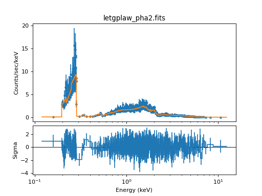
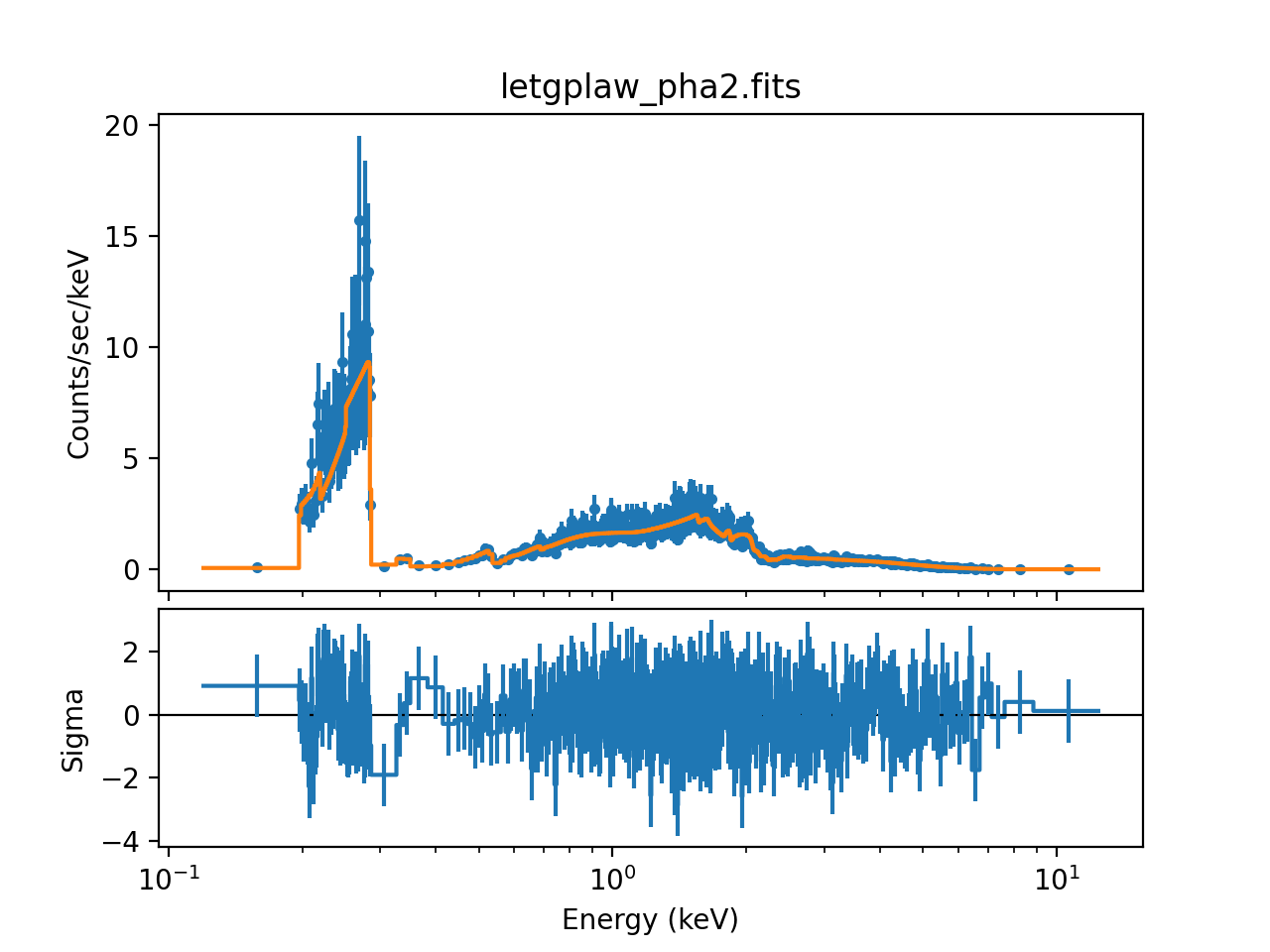
The reduced chi-squared value indicates that we found an acceptable fit and all parameter values are close to the original input values (the nH is so small in the input that the fit may give a zero value as fit result). Note that your results may vary slightly if you run this example, because marx is a Monte-Carlo simulation based on random numbers.
ui.plot_fit_delchi(xlog=True)

Simulated Spectrum in order -1 and a best-fit model.
