Including background in a marx simulation
Chandra observations include different background components: Astrophysical background (e.g. unresolved sources), instrumental background (e.g. high-energy particles from the sun), and a read-out artifact. The Proposers Observatory Guide describes all these components in detail.
The background matters most for faint or extended sources. In this example we show two different methods to include a background component into a marx simulation. Because marx ray-traces X-ray photons and does not calculate the interaction between spacecraft components and energetic particles, both methods need to make approximations:
The Chandra calibration team has released “blank sky background” files for the ACIS detector. Adding “blank-sky background” to a marx simulation shows how to add observed background events from these files to a marx simulation. This should provide the most realistic background, but there are several caveats:
As described in Current caveats for MARX, marx does not incorporate the non-uniformity maps for the ACIS detector, nor does it employ the spatially varying CTI-corrected pha redistribution matrices (RMFs). As such there always will be systematic differences between the simulated MARX source and the real background data.
The “blank sky” files contain between a 30,000 and a few million photons (depending on the chip). If this procedure is repeated for many marx simulations, it adds photons from the same pool every time, so this cannot be used for a statistical analysis if the total number of background photons approaches the number of photons in the file.
We extract and fit the apparent spectrum of the “blank sky” files (“apparent” because the events look like X-ray photons on the CCD, but in reality many are electron or proton impacts) and then use marx to simulate an extended source that produces a similar spectrum (Simulating a background-like source with marx). This approach is easier and faster, but it does not include all spatial variations of the background.
Warning
Background is time variable!
The background count rate can vary within minutes in so-called flares (example for a background lightcurve), and even the quiescent background level changes over time. Thus, the simulation can only give a prediction of a typical background. The actual background might turn out to be higher or lower.
Warning
Sky background depends on Ra, Dec!
See e.g. Markevitch (2002) for a comparison of Chandra and XMM-Newton data of the same galaxy cluster, where the fitted temperature strongly depends on the background model and the Chandra “blank sky” files underpredict the background flux.
Simulating the source: A diffuse, thermal emission
In this example, we model a diffuse emission region with a cool, thermal plasma as they are often seen in massive star forming regions. For the purposes of this example, we do not model the stars themselves, which would show up as additional point sources. We chose a relatively simple model with one thermal emission component in collisional ionization equilibrium with parameters similar to those observed by Güdel et. al (2008) in Orion.
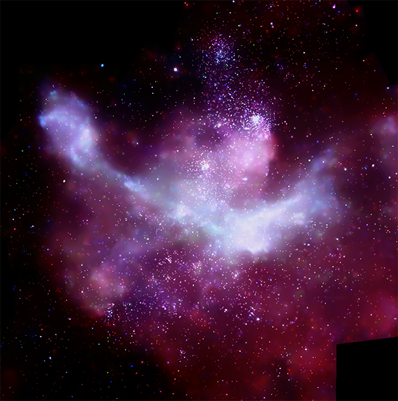
X-rays in the Carina Nebula
Point sources and diffuse emission in the Carina Nebula, yet another star forming region with diffuse emission. The image is a composite from several Chandra observations. Townsley et al. (2011) fit the diffuse emission with a complex model of 6 components, most of which are thermal plasmas.
Image credit: NASA/CXC/PSU/L.Townsley et al.
Similar to Creating an input spectrum from a Sherpa model we will use Sherpa to create a 2-column text file that tabulates the flux density [photons/sec/keV/cm^2] (second column) as a function of energy [keV] (first column).
import numpy as np
from sherpa.astro import ui

# set source properties
ui.set_source(ui.xsphabs.abs1 + ui.xsapec.apec1)
abs1.nH = 0.01
apec1.kT = 0.1

my_src = ui.get_source()

# set energy grid
bin_width = 0.01
energies = np.arange(0.03, 12., bin_width)

# evaluate source on energy grid
flux = my_src(energies)

# Sherpa uses the convention that an energy array holds the LOWER end of the bins;
# Marx that it holds the UPPER end of a bin.
# Thus, we need to shift energies by one bin.
# Also, we need to divide the flux by the bin width to obtain the flux density.
ui.save_arrays("source_flux.tbl", [energies[1:], flux[:-1] / bin_width],
               ["keV","photons/s/cm**2/keV"], ascii=True, clobber=True)
More details about the format of the marx input spectrum can be found at
SpectrumFile.
The next step is to run marx in the desired configuration.
Here, we will wrap the marx call
into a Python script. Since marx currently does not have a “nice” Python
interface, we run it via subprocess.call():
import subprocess
out = subprocess.call('marx SourceFlux=0.001 SpectrumType="FILE" ' + \
         'SpectrumFile="source_flux.tbl" ExposureTime=10000 OutputDir=diffuse ' +\
         'DitherModel="INTERNAL" SourceType="GAUSS" S-GaussSigma=60 ' +\
         'GratingType="NONE" DetectorType="ACIS-S" TStart=2012.5 ' +\
         'RA_Nom=30 Dec_Nom=40 Roll_Nom=0 SourceRA=30 SourceDEC=40', shell=True)
The SourceFlux sets the observed photon flux by renormalizing the input
spectrum. For the shape of the source we choose a Gaussian that is more than one
arcmin wide and we set the aimpoint on the back-illuminated ACIS-S3 chip (chip ID 7). The results of the
simulation will be written to a subdirectory called diffuse, as
specified by the OutputDir parameter. After the simulation has
completed, a standard Chandra event file may be created using the
marx2fits program:
out = subprocess.call('marx2fits diffuse diffuse_evt2.fits', shell=True)
We also generate an aspect solution file that matches the simulation:
out = subprocess.call('marxasp MarxDir="diffuse" OutputFile="diffuse_asol1.fits"', shell=True)
Adding “blank-sky background” to a marx simulation
The “blank sky background” files are part of
CalDB but because of their size
they are not installed by default. If you don’t have them yet, use the
ciao-install script or download them
by hand from http://cxc.harvard.edu/ciao/download/caldb.html . marx does not
simulate all physical effects in Chandra (see Current caveats for MARX) and thus none of
the “blank sky background” files matches the way that marx generates the data
exactly. In particular, marx does not apply the CTI correction, thus we will
use the “blank sky background” files that do not have _cti in their
filename. The naming convention is
acis<chip><aimpoint>D<date>bkgrndN<version>.fits.
In this simulation we care for chip-ID 7 and the ACIS-S aimpoint, so we select the most recent background file and copy it to the working directory:
import os
caldb_bkg = os.environ['CALDB'] + "/data/chandra/acis/bkgrnd/acis7sD2009-09-21bkgrndN0002.fits"
We now need to do some fiddling with the marx simulation and the background file to make their formats compatible so that we can eventually merge them into a single event file. This involves the following steps:
Select a random subset of photons in the “blank sky file”. We need to
Estimate the number of background photons we want to simulate. Looking at the appropriate table in the Observatory Guide we see that roughly 0.3 cts/s (in the event grades we care for) is a good, conservative estimate. For an observation of 100 ks, we thus decide to select roughly 30,000 photons.
Find the number of rows in that file.
Events in the “blank sky” files are sorted in x and y. In order to select a random subset, draw a random number and compare it to the ratio of the number of photons in the “blank sky” file and the number of photons we want to select.
Reproject the “blank sky” file to the observed position on the sky.
Select the same columns in the marx simulation and the “blank sky” file, so that they can be merged with dmmerge.
Here is the script that we use:
n_select=30000

from ciao_contrib import runtool as rt

n = rt.dmlist(caldb_bkg, opt="counts")

rt.dmtcalc(caldb_bkg, "temp.fits", expression=f"randnum={n}/{n_select}*#trand", clobber=True)
rt.dmcopy("temp.fits[randnum=0:1]" , "temp2.fits", clobber=True)

# Assign some random time during the observation to each photon.
t0=float(rt.dmkeypar("diffuse_evt2.fits", "TSTART", echo=True))
t1=float(rt.dmkeypar("diffuse_evt2.fits", "TSTOP", echo=True))

rt.dmtcalc("temp2.fits", "temp3.fits", expression=f"time={t0}+({t1}-{t0})*#trand", clobber=True)
rt.dmsort("temp3.fits", "temp4.fits", keys="TIME", clobber=True)

# Reproject the blank sky fields to the same position on the sky as the marx simulation.
rt.reproject_events.punlearn()
rt.reproject_events(infile="temp4.fits", outfile="acis7s_bkg_reproj.fits",
                    aspect="diffuse_asol1.fits", match="diffuse_evt2.fits", clobber=True)

# Merge marx simulation and blank sky fields into a single fits table.
rt.dmmerge.punlearn()
cols="ccd_id,node_id,chip,det,sky,pha,energy,pi,fltgrade,grade,time"
rt.dmmerge(f"diffuse_evt2.fits[cols {cols}],acis7s_bkg_reproj.fits[cols {cols}]",
            "merged.fits", clobber=True)
rt.dmcopy("merged.fits[energy=200:2000]", "merged_soft.fits", clobber=True)
If the source in the simulation covers multiple ACIS chips, then this has to be repeated chip-by-chip.
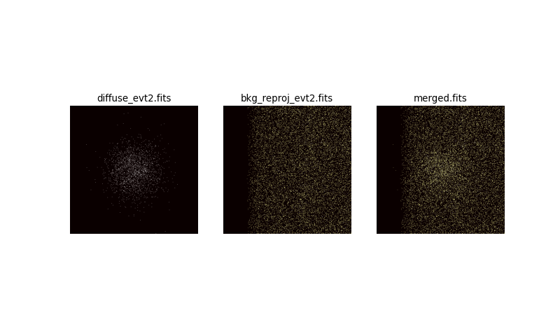
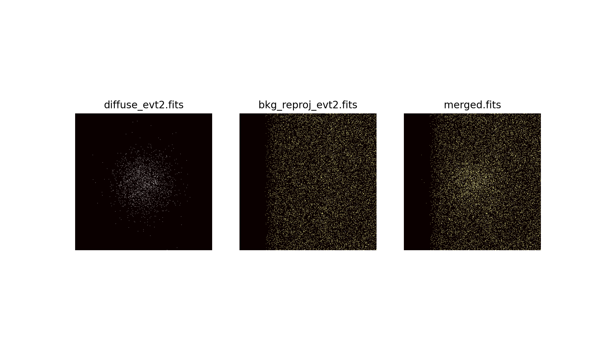
Now, we make a figure to show the marx simulation alone, with added background from the “blank sky” file, and with an energy filter that we would probably use for real data to suppress the background.
import pycrates
import matplotlib.pyplot as plt
from astropy.visualization import PercentileInterval, LogStretch, ImageNormalize

fig, axes = plt.subplots(1, 3, figsize=(10, 2.5), subplot_kw={'aspect':'equal'},
                        sharex=True, sharey=True)
bins = [400, 400]
bin_size = 4
range = [[4096 - 0.5 * bin_size * bins[0], 4096 + 0.5 * bin_size * bins[0]],
        [4096 - 0.5 * bin_size * bins[1], 4096 + 0.5 * bin_size * bins[1]]]
for ax, src in zip(axes, ["diffuse_evt2.fits", "acis7s_bkg_reproj.fits", "merged_soft.fits"]):
    evt = pycrates.read_file(src)
    hist, x, y = np.histogram2d(evt.get_column('X').values, evt.get_column('Y').values,
                                bins=bins, range=range)
    norm = ImageNormalize(hist, interval=PercentileInterval(99), stretch=LogStretch())
    ax.imshow(hist.T, origin='lower', norm=norm, cmap='hot',
            extent=np.array(range).flatten())
    out = ax.set_title(src)
    ax.set_axis_off()

left: Image of the marx simulation alone. The source is extended and not very strong. center: Background added to the simulation. The source is not visible any longer, because the background totally domiantes the count rate. right: We know that our source is fairly soft, while the background contains a lot of high-energy events. Thus, we can apply an energy filter (here 0.2-2.0 keV) that focusses on the energy range where the source is strongest relative to the background. A slight overdensity of photons can be seen at the position of the source, but it will be very difficult to fit spectral parameters or to determine the radius of the source accurately.
The figure shows the marx simulation alone, with added background from the “blank sky” file and with an energy filter that we would probably use for real data to suppress the background.
Looking at the background-free marx simulation, measuring the flux and the size of this source seems like an easy task. When properly including background the source can still be detected, but fitted source parameters will be more uncertain than they would be in a background-free scenario. This example shows how important it is to consider the instrumental background when simulating weak sources.
Simulating a background-like source with marx
An alternative approach is to extract a spectrum from the “blank-sky” fields and use this spectrum as input for marx. This spectrum does not describe the real physical properties such as the energy of the background events (many of them are not even photons), it just provides an effective way to simulate “something that looks similar to real background when run through marx”.
The advantage of this approach is that we can generate more random events than the original “blank-sky” file has without repeating photons.
First, extract a spectrum from the “blank-sky” background and save this spectrum in a table that marx can read. This can be done with the following commands (a detailed explanation for this is at http://cxc.harvard.edu/ciao/threads/extended/ ):
rt.dmextract(infile=f"acis7s_bkg_reproj.fits[sky=rotbox(1:59:59,+39:59:20,3.2',3.5',0)][bin pi]",
        outfile='blank_sky.pi', wmap="[bin tdet=8]", clobber=True)
rt.asphist(infile="diffuse_asol1.fits", outfile="blank_sky.asphist",
        evtfile="diffuse_evt2.fits[ccd_id=7]", clobber=True)
rt.sky2tdet(infile="acis7s_bkg_reproj.fits[sky=rotbox(1:59:59,+39:59:20,3.2',3.5',0)][bin sky=8]",
        asphistfile="blank_sky.asphist",
        outfile="blank_sky_tdet.fits[wmap]", clobber=True)
rt.mkwarf(infile="blank_sky_tdet.fits[wmap]", outfile='blank_sky.arf',
        weightfile='blank_sky.wfef', egridspec="0.3:11.0:0.1",
        mskfile=None, spectrumfile=None, pbkfile=None, clobber=True)
rt.mkrmf(infile="CALDB", outfile="blank_sky.rmf",
        axis1="energy=0:1", axis2="pi=1:1024:1", weights="blank_sky.wfef", clobber=True)
We use Sherpa to display the spectrum on the screen and save it in a table
with columns energy and count rate density (see SpectrumFile for details
of the input spectrum format for marx):
from sherpa.astro import ui

ui.load_data('blank_sky.pi')
ui.load_rmf('blank_sky.rmf')
ui.load_arf('blank_sky.arf')
ui.plot_data()

pl = ui.get_data_plot()
ui.save_arrays('bkgspec.tbl', [pl.x, pl.y], ['Energy', pl.ylabel],
               ascii=True, clobber=True)
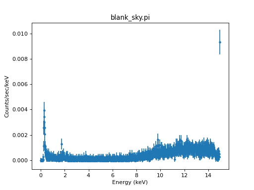
Spectrum of the “blank-sky” background.
Again, we want a source flux of about 0.3 counts/s over the entire detector.
SourceFlux expects the flux in counts/s/cm^2, so we would have to devide
by Chandra’s effective area. Alternatively, we can just set the
exact number of photons we want to detect with ExposureTime=0 and NumRays
set to a negative number. We set SpectrumFile to the spectrum of
the background. Now we only need to specify the shape of the
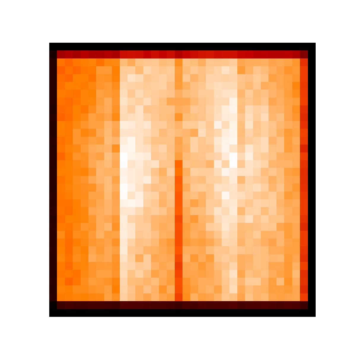
source. The figure with the chip backgorund shows regions with higher or
lower background level in the input “blank sky” file.
rt.dmcopy(f"{caldb_bkg}[EVENTS][bin x=3850:4930:32,y=3550:4650:32]",
          "chip-shape.fits", clobber=True)

im = pycrates.read_file("chip-shape.fits")
fig, ax = plt.subplots(figsize=(6,6), subplot_kw={'aspect':'equal'})
ax.imshow(im.get_image().values, origin='lower', cmap='gist_heat')
ax.set_axis_off()
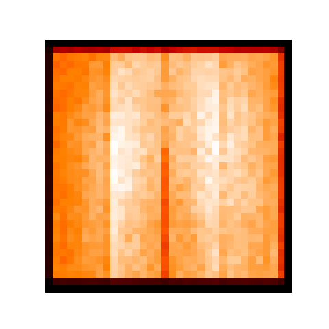
Binned “blank sky” file for chip 7
To reproduce this pattern, we use marx with SourceType="IMAGE".
There is a trade-off here: If we bin the image too much, we smooth out the
structure, if we bin too little such that we still see the random noise in the
image, then our marx simulation will produce an event distribution that shows
the same “random noise pattern”. That fine, unless we want to run many marx
simulations, where we would see the same “random” pattern again and again. Here, the
binning is chosen such that we find a few thousand events in every pixel of the
image.
All remaining marx parameters (RA_Nom, Dec_Nom etc.) are the
same as in the simulation of the astrophysical source of interest above.
out = subprocess.call('marx SourceFlux=3. SpectrumType="FILE" SpectrumFile="bkgspec.tbl" ' + \
   'ExposureTime=0 NumRays=-30000 TStart=2012.5 OutputDir=bkg ' + \
   'DetectorType="ACIS-S" DitherModel="INTERNAL" RA_Nom=30 Dec_Nom=40 ' + \
   'Roll_Nom=0 SourceRA=30 SourceDEC=40 GratingType="NONE" ' + \
   'SourceType="IMAGE" S-ImageFile="chip-shape.fits"', shell=True)
Now, we can use marxcat to merge the simulation of the diffuse
source and the background and marx2fits to convert the merged
results into a fits file.
out = subprocess.call('marxcat diffuse bkg diffuse_with_bkg', shell=True)
out = subprocess.call('marx2fits diffuse_with_bkg diffuse_with_bkg.fits', shell=True)
rt.dmcopy("diffuse_with_bkg.fits[energy=200:2000]", "diffuse_with_bkg_soft.fits", clobber=True)
fig, axes = plt.subplots(1, 3, figsize=(10, 2.5), subplot_kw={'aspect':'equal'},
                        sharex=True, sharey=True)
bins = [400, 400]
bin_size = 4
range = [[4096 - 0.5 * bin_size * bins[0], 4096 + 0.5 * bin_size * bins[0]],
        [4096 - 0.5 * bin_size * bins[1], 4096 + 0.5 * bin_size * bins[1]]]
for ax, src in zip(axes, ["diffuse_evt2.fits", "diffuse_with_bkg.fits", "diffuse_with_bkg_soft.fits"]):
    evt = pycrates.read_file(src)
    hist, x, y = np.histogram2d(evt.get_column('X').values, evt.get_column('Y').values,
                                bins=bins, range=range)
    norm = ImageNormalize(hist, interval=PercentileInterval(99.), stretch=LogStretch())
    ax.imshow(hist.T, origin='lower', norm=norm, cmap='hot',
            extent=np.array(range).flatten())
    out = ax.set_title(src)
    ax.set_axis_off()

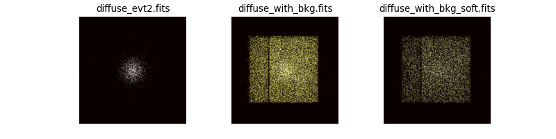
Images of the event files with marx simulated background
This figure has the same panels as the figure for adding photons directly from the background file, except that the background is simulated with marx here.
Looking at the figure here we again see that the background makes it much harder to discern the source. The images look very similar to first method, indicating that both approaches to describe the background give similar results. The main difference is that in the marx simulation the edge of the chip is more fuzzy. That’s because pixel boundaries in the image of the chip background do not coincide exactly with the chip boundaries and thus we simulate the “background” for a region slightly larger than the chip. However, this is not important for our purpose: Finding how well we can fit the source position, size and spectrum in the presence of background.
Notes about additional background components
In addition to the instrumental background, there is also an astrophyiscal background. This can be unrelated to the target of the observation, such as charge exchange emission in the solar wind or the population of weak background AGN, that is roughly homogeneous over the field-of-view and contributes to the observed “diffuse” background.
For some targets, there are additional contributions to the apparent background that are related to the source. For example, in the case of diffuse emission in a star forming region there will be stars in the cluster. While the bright stars should be detected as point sources and those regions can be excluded from the analysis, there might be a population of weak stars that contribute only a few photons each, but add up to provide significant flux in addition to a truly diffuse component from a hot gas.
Different strategies can be used to account for those backgrounds in spectral modeling, but that is beyond the scope of this marx example.
