Replicating a Chandra Observation / Using ChaRT or SAOTrace¶

The example presented here was originally designed to see how well the marx PSF compares to that of an actual Chandra observation of a far off-axis source. We will also be comparing the marx intrinsic PSF to that of SAOTrace (SAOTrace is a high-fidelity ray-tracer for the Chandra mirrors that simulates many details that are treated statistically in marx to improve efficiency). Hence, this example will serve several purposes:

How to simulate an existing observation.
How to use SAOTrace dithered rays with marx.
To see how the SAOTrace and marx PSFs compare to the observed PSF for a far off-axis source.

In this example, we will use the 1999 Chandra calibration observation of LMC X-1 observed about 25 arc-minutes off-axis with the ACIS detector (ObsID 1068). We download the data with download_chandra_obsid. If we want to be sure that the newest calibration data has been applied we could also reprocess it with chandra_repro but this particular observation is old enough that the calibration does not change any longer.

We can look at the event file in ds9 to find the coordinates that we are interested in or look at plot in Python:

from matplotlib import pylab as plt
import matplotlib.colors as colors

from ciao_contrib.cda.data import download_chandra_obsids
import pycrates

out = download_chandra_obsids([1068], filetypes=['evt2', 'asol'])

asolfile = '1068/primary/pcadf01068_000N001_asol1.fits.gz'
evt2file = '1068/primary/acisf01068N004_evt2.fits.gz'

x, y = 5256, 6890

evt = pycrates.read_file(evt2file)

fig, ax = plt.subplots(1, 1, figsize=(6,6), subplot_kw={'aspect':'equal'})
out = ax.hist2d(evt.get_column('X').values, evt.get_column('Y').values,
                bins=[200, 200], range=[[x-150,x+150], [y-150,y+150]],
                    cmap='hot_r', norm=colors.LogNorm(vmin=1, vmax=15))
ax.plot(x, y, 'b+', markersize=30, markeredgewidth=3)
ax.set_axis_off()
_ = plt.colorbar(out[3], ax=ax, label='Counts / bin')

(png, hires.png, pdf)

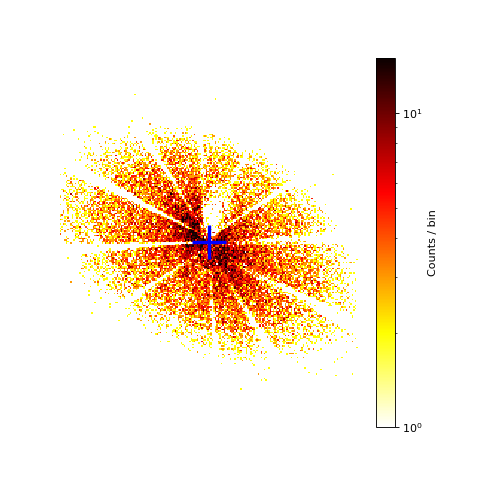
The Chandra PSF at this position is an ellipse with spokes. — Image of the PSF for a bright off-axis source in ObsID 1068¶

The blue cross in the image marks the position where the support strut shadows meet as determined by eye: ra=84.91093 degrees, dec=-69.74348 degrees, (x,y)=(5256,6890). This coordinate will be used as the position of the source. For this observation, this coordinate falls on chip ACIS-4 (S0).

Creating the source spectral file¶

For an accurate simulation of an observed source, it is important to make the detector configuration match that of the observation as closely as possible. And since the PSF is energy dependent, a rough idea of the energy dependence of the incident source flux must be obtained. There are several approaches to get this input spectrum. One way would be to extract the spectrum, fit a model using XSPEC, ISIS, or Sherpa and write an input file from the model as we did in several previous examples.

Just to illustrate another approach, we will do something different here. (But do not worry if that looks like black magic to you; you can get the input spectrum from a spectral fit, too. We just think it is instructive to show something slightly different in each example.)

Here, we will simply extract the counts in a region containing the observed PSF and divide it by the effective area. This is known as “flux-correction”, and involves no spectral fitting. Strictly speaking, the validity of this technique assumes that the spectrum does not vary much over the scale of the RMF.

The first step is to create the ARF to be used for the flux-correction. The creation of the ARF is straightforward via this script:

import ciao_contrib.runtool as rt

aspfile="obs1068.asp"
arffile="obs1068.arf"

rt.asphist(infile=asolfile, outfile=aspfile, evtfile=evt2file, clobber=True)

# It would be more accurate to use mkwarf.
# However, that's slower and for our purposes an approximate solution is good enough.
rt.mkarf(detsubsys="ACIS-S0", grating="NONE", outfile=arffile,
        obsfile=evt2file, asphistfile=aspfile,
        sourcepixelx=x, sourcepixely=y, engrid="0.3:8.0:0.1",
        maskfile="NONE", pbkfile="NONE", dafile="NONE", clobber=True)

The next step is to extract the counts in the PSF and divide by the ARF to get the flux corrected spectrum. Here we show a way using only standard CIAO tools and Python packages that are part of the CIAO distribution.

First, create a region file containing the source events with dmellipse, and use dmextract to create the PI histogram.

rt.dmcopy(f"{evt2file}[EVENTS][bin x=4950:5530:1,y=6700:7100:1]", "image.fits",
        option="image", clobber=True)
rt.dmellipse("image.fits", "psf90.reg", 0.9, clobber=True)

# We have to use the same energy binning in energy space here that we used for the arf!
# So, first convert the PI to energy (to a precision that's good enough for this example.)
rt.dmtcalc(f"{evt2file}[EVENTS][sky=region(psf90.reg)]", "obs1068_evt2_with_energy.fits",
            expr="energy=(float)pi*0.0149", clobber=True)
rt.dmextract("obs1068_evt2_with_energy.fits[bin energy=.3:7.999:0.1]", "obs1068.spec",
            clobber=True, opt="generic")

The energy binning of the ARF and extracted spectrum are the same. Thus, we can now calculate the corrected spectrum by dividing the flux by the effective area and exposure time. There is an extra factor of 0.9, because the ARF assumes that 100% of the PSF are included in the data extraction, while the ellipse above only contains 90% of the counts. Also, we divide by the exposure time (about 1760 s).

arf = pycrates.read_file(arffile)
spec = pycrates.read_file("obs1068.spec")

flux = spec.get_column('COUNTS').values / arf.get_column('SPECRESP').values / (0.9 * 1759.8)


with open('input_spec_marx.tbl', 'w') as f:
    f.write('# KEV PHOTONS/S/CM**2/KEV\n')
    for a,b in zip(arf.get_column('ENERG_HI').values,
                   # divide by bin width to get flux density
                   flux / 0.1):
        f.write(f"{a} {b}\n")

# SAOTrace requires input in tab-limited rdb format.
with open('input_spec_saotrace.rdb', 'w') as f:
    f.write('ENERG_LO\tENERG_HI\tFLUX\n')
    for a,b,c in zip(arf.get_column('ENERG_LO').values,
                     arf.get_column('ENERG_HI').values,
                     flux):
        f.write(f"{a}\t{b}\t{c}\n")

The resulting ASCII tables with the spectrum will be input into both marx and SAOTrace. The spectrum is the same, but the format of the tables is two columns (energy, flux density) for marx and three columns (lower energy, upper energy, flux) for SAOTrace / ChaRT.

Running marx (without SAOTrace)¶

Running marx for this example does not differ much from any of the previous examples. We use the SpectrumFile parameter to input the source spectrum we estimated above and set the remaining parameters to match the setting of the observation for the pointing direction, exposure time, etc. To get the numbers we can either display the header (e.g. in ds9) and manually look for the required fits header keywords (e.g. EXPOSURE for ExposureTime, RA_NOM for RA_Nom, etc.) or extract the values using dmkeypar. Note that TStart is given in seconds on the spacecraft clock here as in the TSTART and TSTOP header keywords. However, for some ObsIDs, the TSTART time is set to include some spacecraft slew before the actual observation starts. marx can deal with a start time set slightly before the data in the aspect solution file (asol file) starts, but SAOTrace will raise an error. Thus, we set the start time of the simulation to the first entry in the asol file.

import gzip
import shutil
import subprocess

# marx cannot read gzipped asol files, so unzip
asolfile_unzipped = asolfile[:-3]
with gzip.open(asolfile, 'rb') as f_in:
    with open(asolfile_unzipped, 'wb') as f_out:
        shutil.copyfileobj(f_in, f_out)
asolfile = asolfile_unzipped

ra_nom = float(rt.dmkeypar(infile=evt2file, keyword="RA_NOM", echo=True))
dec_nom = float(rt.dmkeypar(infile=evt2file, keyword="DEC_NOM", echo=True))
roll_nom = float(rt.dmkeypar(infile=evt2file, keyword="ROLL_NOM", echo=True))
exptime = float(rt.dmkeypar(infile=evt2file, keyword="EXPOSURE", echo=True))

# Get time of first entry in asol file
asol = pycrates.read_file(asolfile)
tstart = asol.get_column('time').values[0]
# Add a little offset in case of rounding errors when reading the file.
tstart += 0.1

# We will run marx more than once, so make a string that contains the common parameters.
marx_with_parameters = f"marx ExposureTime={exptime} TStart={tstart} " + \
    "GratingType='NONE' DetectorType='ACIS-S' " + \
    f"RA_Nom={ra_nom} Dec_Nom={dec_nom} Roll_Nom={roll_nom} " + \
    "SourceRA=84.91093 SourceDEC=-69.74348 " + \
    f"DitherModel='FILE' DitherFile='{asolfile}' " + \
    "SourceFlux=-1 SpectrumType='FILE' "

# Combine common parameters with the ones specific to this run.
subprocess.call(marx_with_parameters + \
                "SpectrumFile='input_spec_marx.tbl' OutputDir='marx_only'", shell=True)

subprocess.call("marx2fits marx_only marx_only.fits", shell=True)

Running SAOTrace / Chart and marx¶

SAOTrace is a high fidelity ray-trace of the Chandra mirrors, which simulates details of the mirror roughness and alignment that are only approximated in marx because these details are not important for almost all Chandra simulations and they require a much longer run time.

SAOTrace is a separate, stand-alone program that you need to download and install following the instructions in the SAOTrace documentation at http://cxc.harvard.edu/cal/Hrma/Raytrace/SAOTrace.html. Alternatively, you can use ChaRT, which is a web interface to SAOTrace. Using ChaRT saves you the installation, but it is less flexible (e.g. it can only simulate single sources).

Below, we use a locally installed version of SAOTrace, but to follow this example, you can equally well upload input_spec_saotrace.rdb to ChaRT. SAOTrace itself is a very complex system of many different parts. Here, we will explain the parameters used in this example, but we need to refer to the SAOTrace documentation for details.

We define the source in a file called saotrace_source.lua:

ra_pnt = 85.368613
dec_pnt = -70.12585
roll_pnt = 116.86955

dither_asol_chandra{ file = "1068/primary/pcadf01068_000N001_asol1.fits",
                     ra = ra_pnt, dec = dec_pnt, roll = roll_pnt }

point{ position = { ra = 84.91093,
          dec = -69.74348,
          ra_aimpt = ra_pnt,
          dec_aimpt = dec_pnt,
       },
       spectrum = { { file = "input_spec_saotrace.rdb", 
                      units = "photons/s/cm2", 
                      scale = 1, 
                      format = "rdb",
                      emin = "ENERG_LO",
                      emax = "ENERG_HI",
                      flux = "FLUX"} }
    }

and run SAOTrace with the following command:

subprocess.run(f"trace-nest tag=saotrace srcpars=saotrace_source.lua tstart={tstart} " + \
               f"limit={exptime} limit_type=sec", shell=True)

This gives us a ray file called saotrace.fits. We take this file as input for marx using SourceType="SAOSAC" and SAOSACFile="saotrace.fits". All the remaining parameters for the exposure time, pointing direction etc. are the same as above:

subprocess.call(marx_with_parameters + \
                "SourceType='SAOSAC' SAOSACFile='saotrace.fits' " + \
                "OutputDir='marx_saotrace'", shell=True)

subprocess.call("marx2fits marx_saotrace marx_saotrace.fits", shell=True)

Comparing the results¶

We can now use ds9 to compare the observation with the two simulated event lists or plot them with matplotlib:

fig, axes = plt.subplots(1, 3, figsize=(10,3), subplot_kw={'aspect':'equal'})
for ax, src, title in zip(axes.flatten(),
                [evt2file, "marx_only.fits", "marx_saotrace.fits"],
                ['Observation', 'MARX only', 'SAOTrace + MARX']):
    evt = pycrates.read_file(src)
    out = ax.hist2d(evt.get_column('X').values, evt.get_column('Y').values,
                    bins=[200, 200], range=[[x-150,x+150], [y-150,y+150]],
                    cmap='hot_r', norm=colors.LogNorm(vmin=1, vmax=15))
    out = ax.set_title(title)
    ax.set_axis_off()
fig.subplots_adjust(wspace=0)

(png, hires.png, pdf)

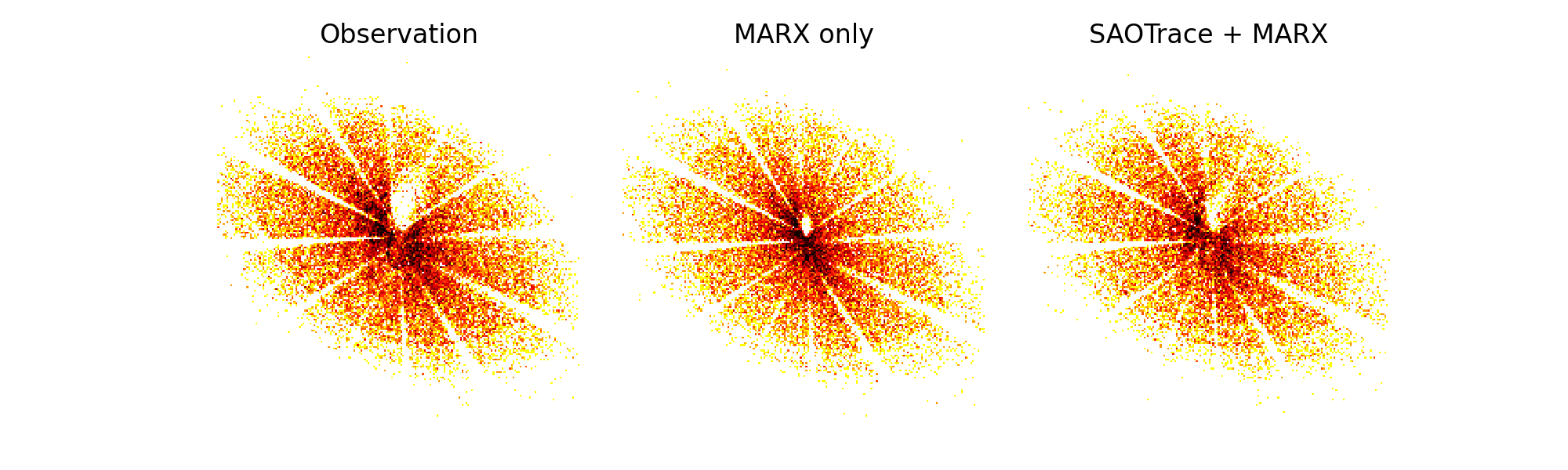
Three very similar PSFs. — Comparison of the observed PSF with the two simulations.¶

The structure of the PSFs is very similar, emphasizing how good both mirror models are. On closer inspection, there is a small shadow just above and to the right of the point where the support strut shadows meet. This feature is a little smaller in marx than in SAOTrace or the real data due to the simplification that the marx mirror model makes. However, very few point sources are observed long enough this far off-axis that these tiny differences actually matter.

So, we can see from this comparison that marx is the tool of choice for almost all Chandra simulations.

Replicating a Chandra Observation / Using ChaRT or SAOTrace¶

Creating the source spectral file¶

Running marx (without SAOTrace)¶

Running SAOTrace / Chart and marx¶

Comparing the results¶

Page Content

Previous topic

Next topic