Simulating two overlapping sources
In each run of marx the user can choose one and only one source from the list in The spectrum and the spatial shape of the X-ray source. Most of these sources are simple geometric shapes like a point or a disk. The IMAGE Source allows the user to specify an intensity image as input to define a complicated morphology on the sky, but the spectrum is the same in every position.
If spectrum and intensity change with position, the user can write his/her own C-code to generate the photons as described in USER Source. Some of those codes are available for download, see The spectrum and the spatial shape of the X-ray source for links. The SIMPUT Source can also be used for complex input sources, but it requires the user to install the SIMPUT code and write a source specification according to the SIMPUT standard.
However, in most cases it is easier to run marx several times and use marxcat to combine the simulations.
In this example we want to simulate a binary star, where both components are separated by only a few arcseconds. In the center of the field-of-view that is enough to separate the images of component A and B, but what happens when we insert a grating? Will the dispersed spectra overlap, or can they be separated in the data?
The parameters in the following example are inspired by the observations of the M-dwarf binary EQ Peg (ObsID 8453). An analysis is presented by Liefke et al. (2008). We will run two marx simulations, one for EQ Peg A and one for EQ Peg B. The parameters of the observations (pointing coordinates, roll angle, exposure time, grating) have to be the same for both simulations, but the parameters for the sources (coordinates, count rate, spectrum) are different.
Creating a file with the input spectra
First, we need to generate the input spectra. For this example, we use Sherpa, but XSPEC or ISIS work very similar. We need two 2-column text files that tabulate the model flux [photons/sec/keV/cm^2] (second column) as a function of energy [keV] (first column).
Stars are generally well described by an optically thin, collisionally excited plasma. We use a model with only a single temperature component with a different temperature for EQ Peg A and EQ Peg B and slightly non-solar abundances as suggested by Liefke et al. (2008).
import numpy as np
from sherpa.astro import ui
# set source properties
ui.set_source(ui.xsvapec.a1)
a1.Ne = 1.2
a1.Fe = 0.8

# get source
my_src = ui.get_source()

# set energy grid
bin_width = 0.01
energies = np.arange(0.15, 12., bin_width)

### EQ Peg A ###
# We could download and take number from the observed data,
# but that would make for a longer example.
a1.norm = 0.001
a1.kT = 0.95
# evaluate source on energy grid
flux = my_src(energies)

# Sherpa uses the convention that an energy array holds the LOWER end of the bins;
# Marx that it holds the UPPER end of a bin.
# Thus, we need to shift energies by one bin.
# Also, we need to divide the flux by the bin width to obtain the flux density.
ui.save_arrays("EQPegA_flux.tbl", [energies[1:], flux[:-1] / bin_width],
               ["keV","photons/s/cm**2/keV"], ascii=True, clobber=True)

### EQ Peg B ###
a1.norm = 0.0003
a1.kT = 0.7
flux = my_src(energies)

ui.save_arrays("EQPegB_flux.tbl", [energies[1:], flux[:-1] / bin_width],
               ["keV","photons/s/cm**2/keV"], ascii=True, clobber=True)
More details about the format of the marx input spectrum can be found at SpectrumFile.
Running marx
We run marx twice - once for each star.
import subprocess
obssetup = 'ExposureTime=5e5 TStart=2006.9 GratingType="HETG" DetectorType="ACIS-S" ' + \
            'DitherModel="INTERNAL" RA_Nom=352.966 Dec_Nom=19.935 Roll_Nom=290 ' + \
            'SourceFlux=-1 SpectrumType="FILE"'
out_a = subprocess.call('marx SourceRA=352.96851 SourceDEC=19.937133 ' + \
                        'SpectrumFile="EQPegA_flux.tbl" OutputDir=EQPegA ' + obssetup,
                        shell=True)
out_b = subprocess.call('marx SourceRA=352.97011 SourceDEC=19.937225 ' + \
                        'SpectrumFile="EQPegB_flux.tbl" OutputDir=EQPegB ' + obssetup,
                        shell=True)
The SourceFlux parameter may be used to indicate the integrated flux of
the spectrum. The value of -1 means that the integrated flux is taken
from the file. The results of the simulation will be written to sub-directories
called EQPegA and EQPegB, as specified by the OutputDir
parameter. We use marxcat to combine both simulations in the
directory EQPeg_both:
subprocess.call('marxcat EQPegA EQPegB EQPeg_both', shell=True)
In the simulation we know exactly which photon comes from which star, so we can generate three fits files, one for EQ Peg A only, one for EQ PEg B only, and one that contains both sources, similar to the observed data.
subprocess.call('marx2fits EQPegA EQPegA.fits', shell=True)
subprocess.call('marx2fits EQPegB EQPegB.fits', shell=True)
subprocess.call('marx2fits EQPeg_both EQPeg_both.fits', shell=True)
The fits files can be further processed
with standard CIAO tools. As some of these tools require the aspect
history, the marxasp program is used to create an aspect
solution file. Since both simulations used the same pointing and dither, we can
use the same asol file for all three fits files.
subprocess.call('marxasp MarxDir="EQPegA" OutputFile="EQPeg_asol1.fits"', shell=True)
Analyzing the results
It is interesting to look at the event file with a viewer such as ds9 or make a plot. The grating spectra of EQ Peg A and EQ Peg B are close to each other on the detector, and we’ll now test if the spectrum of EQ Peg A contaminates the spectrum of EQ Peg B.
from matplotlib import pyplot as plt
import pycrates
from astropy.visualization import PercentileInterval, LogStretch, ImageNormalize

fig, ax = plt.subplots(1, 1, figsize=(10,6), subplot_kw={'aspect':'equal'})
bins = [400, 200]
bin_size = 4
range = [[4096 - 0.5 * bin_size * bins[0], 4096 + 0.5 * bin_size * bins[0]],
        [4400 - 0.5 * bin_size * bins[1], 4400 + 0.5 * bin_size * bins[1]]]
evt = pycrates.read_file('EQPeg_both.fits')
hist, x, y = np.histogram2d(evt.get_column('X').values, evt.get_column('Y').values,
                            bins=bins, range=range)
norm = ImageNormalize(hist, interval=PercentileInterval(99.9), stretch=LogStretch())
ax.imshow(hist.T, origin='lower', norm=norm, cmap='hot',
        extent=np.array(range).flatten())
ax.set_axis_off()

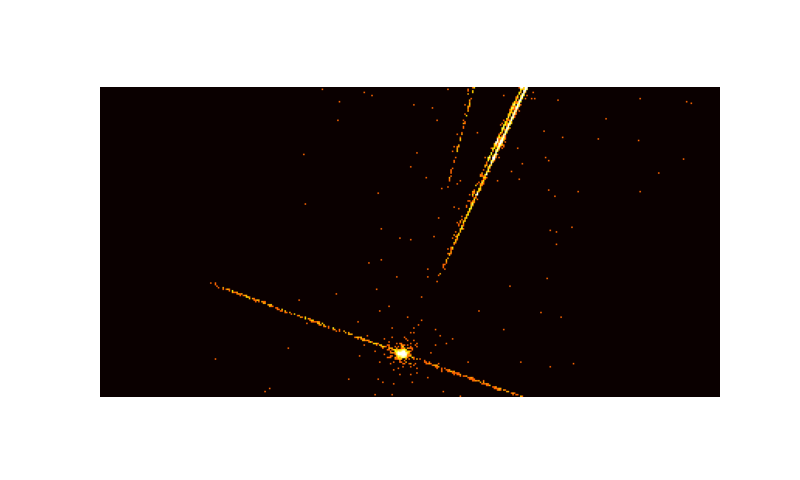
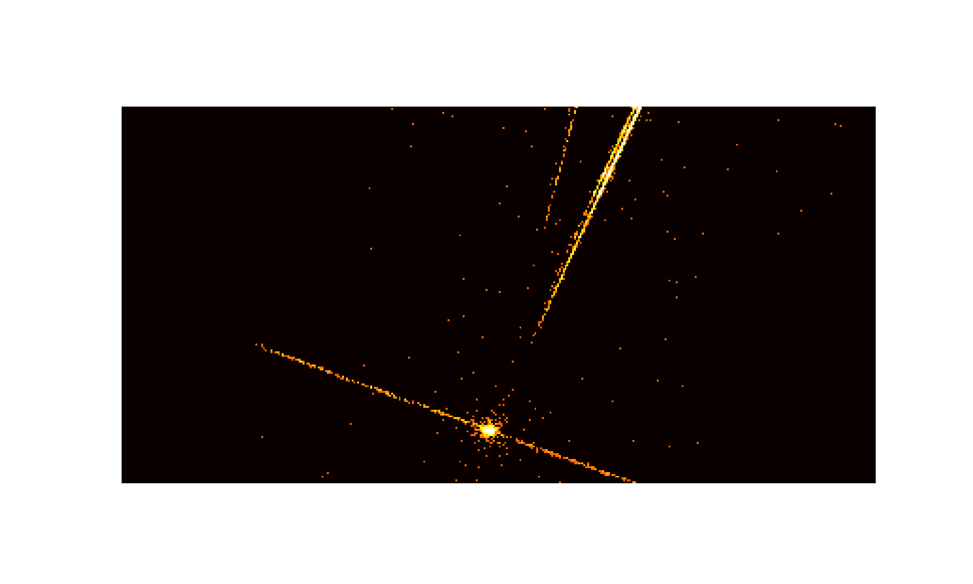
Small section of the detector image of the combined simulation
The grating spectra of both sources are located fairly close to each other. On the top right is an MEG arm, the fainter signal of an HEG arm is seen on the top left. The streak running mostly from left to right with a slight downward slope is the read-out streak.
We use CIAO to extract the grating spectrum from EQPegB.fits and
EGPeg_both.fits.
import ciao_contrib.runtool as rt

# determined by hand in ds9 to make sure we pick the fainter source
X=4068.3
Y=4112.7

# We'll use the same mask for both extractions, because we want the same region.
rt.tg_create_mask(infile="EQPegB.fits", outfile="EQPegB_reg1a.fits",
                  use_user_pars=True, last_source_toread='A',
                  sA_id=1, sA_zero_x=X, sA_zero_y=Y, clobber=True,
                  grating_obs="header_value", width_factor_hetg=10,
                  # see https://github.com/cxcsds/ciao-contrib/issues/1016
                  # on why the following parameters are set to zero
                  # (which means "default") here
                  sA_zero_rad=0, sA_width_heg=0, sA_width_meg=0)


### Extract EQ Peg B from the "EQ Peg B only" simulation ###

rt.tg_resolve_events(infile="EQPegB.fits", outfile="EQPegB_evt1a.fits",
                     regionfile="EQPegB_reg1a.fits", acaofffile="EQPeg_asol1.fits",
                     osipfile="CALDB", verbose=0, clobber=True)

rt.tgextract(infile="EQPegB_evt1a.fits", outfile="EQPegB_pha2.fits",
             tg_order_list="-1,+1", clobber=True)

### Extract EQ Peg B from the combined simulation ###

rt.tg_resolve_events(infile="EQPeg_both.fits", outfile="EQPegB_both_evt1a.fits",
                     regionfile="EQPegB_reg1a.fits", acaofffile="EQPeg_asol1.fits",
                     osipfile="CALDB", verbose=0, clobber=True)

rt.tgextract(infile="EQPegB_both_evt1a.fits", outfile="EQPegB_both_pha2.fits",
             tg_order_list="-1,+1", clobber=True)

# make response matrices for the MEG +1 order
# In practice, one would of course create arf and rmf files for all orders
# but for this example one is enough (to make it faster to run the code).
# We are extracting the exact same region in both cases above for EXACTLY the same
# observational parameters (aimpoint, exposure time, ...).
# Thus the arf and rmf files will be identical, so we have to run this only once.
pharow = 4  # MEG +1 order
order = +1

rt.mkgrmf(grating_arm="MEG", order=order, outfile=f"eqpeg_meg{order}_rmf.fits",
            srcid=1, detsubsys="ACIS-S3", obsfile="EQPegB_pha2.fits",
            regionfile="EQPegB_pha2.fits",
            wvgrid_arf="compute", wvgrid_chan="compute", clobber=True)

# fullgarf produces a lot of output. Let's capture that in a variable in case we need it.
out = rt.fullgarf(phafile="EQPegB_pha2.fits", pharow=pharow,
                    evtfile="EQPegB.fits", asol="EQPeg_asol1.fits",
                    engrid=f"grid(eqpeg_meg{order}_rmf.fits[cols ENERG_LO,ENERG_HI])",
                    maskfile="NONE", dafile="NONE", dtffile="NONE", badpix="NONE",
                    rootname="eqpeg", clobber=True,
                    ardlibqual=";UNIFORM;bpmask=0")
Note that we use ardlibqual=";UNIFORM;bpmask=0" in fullgarf because marx does not simulate QE maps or bad pixels.
Now, we want to make use of our marx simulation to see how much the spectrum
of EQ Peg A contaminates the extracted grating spectrum of EQ Peg B.
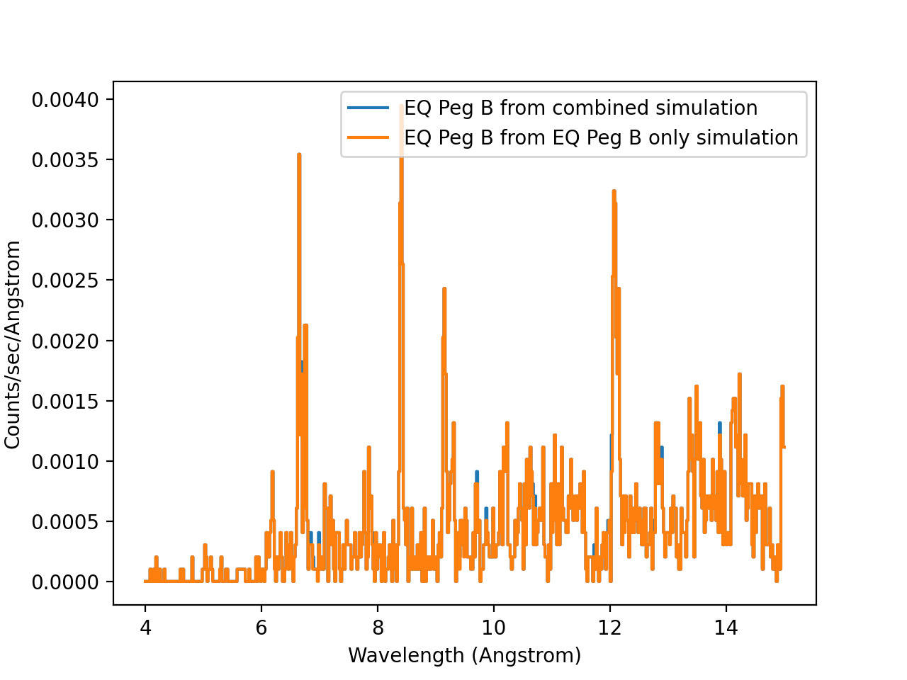
We compare the spectra in Sherpa. The difference between the two spectra in
some of the lines is caused by photons from EQ Peg A that fall in the
extraction region of EQ Peg B.
ui.load_data('EQPegB_both_pha2.fits')
ui.load_arf(4, 'eqpegMEG_1_garf.fits')
ui.load_rmf(4, 'eqpeg_meg1_rmf.fits')
# Load all spectra from pha2file (HEG-1, HEG+1, MEG-1, MEG+1)
# And label them with is 11, 12, 13, 14
ui.load_data(11, 'EQPegB_pha2.fits')
ui.load_arf(14, 'eqpegMEG_1_garf.fits')
ui.load_rmf(14, 'eqpeg_meg1_rmf.fits')
for i in [4, 14]:
    ui.set_analysis(i, 'wave')
    ui.ignore_id(i, None, 4.)
    ui.ignore_id(i, 15., None)
    ui.group_width(i, 4)

ui.plot_data(4, linestyle='solid', yerrorbars=False, marker=None,
             label='EQ Peg B from combined simulation')
ui.plot_data(14, overplot=True, linestyle='solid', yerrorbars=False, marker=None,
             label='EQ Peg B from EQ Peg B only simulation')

plt.legend()
plt.title("")
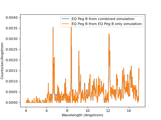
Contaminated and clean spectrum extracted for EQ Peg B (MEG order +1).
Looking at this figure, we see that both spectra are very similar, but not identical - that is the contamination by EQ Peg A.
tgextract uses only the innermost part of the extraction region for the source spectrum and apparently that is narrow enough to avoid most of the contamination. Still, if we want to measure or fit lines in the EQ Peg B spectrum we have to be careful.
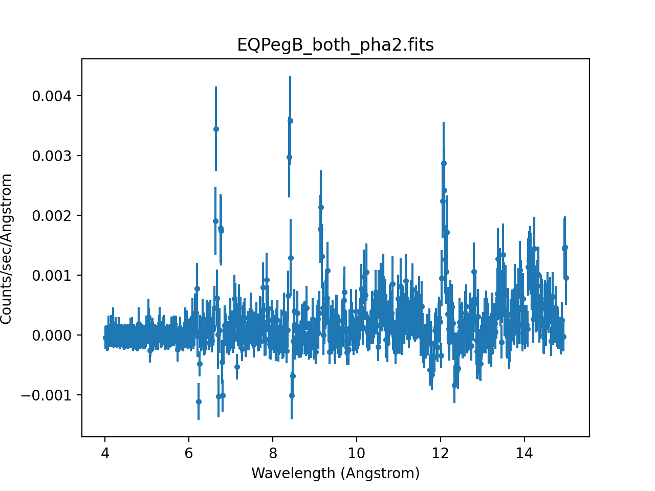
marx simulations do not contain any background, but real data does and one common (although arguably not the best) approach is to subtract a background spectrum from the data. What would happen if we blindly subtracted the background from the EQ Peg B spectrum?
ui.subtract(4)
ui.plot_data(4)

“Background subtracted” spectrum for EQ Peg B
We end up with a spectrum with a significant number of negative bins because the much brighter spectrum of EQ Peg A falls in the region where tgextract extracts the background, leading to an overestimate of the background.
Summary
This example shows how marxcat can be used to build up a more complex distribution of sources on the sky from simple components. We can asses how much the sources overlap and compare the simulated spectra of each component and thus estimate the contamination in the real data.
In this example we simulated grating spectra of a binary star, but the same principle works for all cases where sources overlap on the detector, e.g. a cluster of galaxies with a foreground HMXB, binary AGN, or imaging of a dense star forming region.
