Reproducing an input spectrum
marx allows users to specify either a flat input spectrum or to pass in a file. Here, we generate input spectra with the spectral modeling program Sherpa. We run marx to simulate a point source and extract the data from that simulation using CIAO, read it back into Sherpa and fit the simulated data. If everything works well and all detector effects are treated consistently, we should recover the same spectral parameters (up to Poisson noise). On the other hand, if marx and CIAO are inconsistent the fit parameters will deviate from the input parameters.
In the past, this has happened after the release of marx 5.0, which contains some files to describe the ACIS contamination. This contamination changes with time and several CalDB releases had happened before we released marx 5.1. At that time, marx always predicted too many counts at low energies.
The following tests are designed to test consistency with CIAO. Since there is always some uncertainty about the intrinsic spectrum of astrophysical sources, this test is best done with simulated input spectra.
Absorbed powerlaw on ACIS-S
This test checks the internal consistency of a simulated marx spectrum by simulating a source placed on a back-illuminated chip of ACIS-S. The input spectrum is an absorbed powerlaw.
We generate an input spectrum and run marx. We then extract the spectrum in two different ways:
We use CIAO tools, but specify special qualifiers to account for the fact that marx does not include ACIS QE maps and uses FEF rmfs (FEF’s are parameterized functions to describe the shape of the RMF. They are faster to compute, but not as accurate as the tabulated values usually used in CIAO). We do that by setting the detector name to
"ACIS-7;UNIFORM;bpmask=0"in mkarf and by passing the appropriate FEF to mkrmf.We use the specextract tool without any special qualifiers. While
specextracthas a number of parameters, it does not allow us to set the dectector or force the use of an FEF file. It requires only a call to a single tool, but is inconsistent with the simulations done by marx, so fitted spectra will not match the input parameters as well as in method 1.
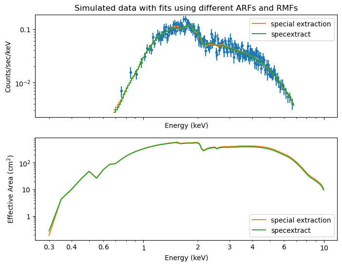
top: Simulated data and two model fits, assuming different ARFs and RMFs. “Special extraction” uses special qualifiers to match marx simulations, while “specextract” uses standard CIAO tools without any special qualifiers.
bottom: Shape of the ARFs used in the two extractions. Since the ARF is different, the model values are different when fitting to the same data (e.g. where the ARF is lower, the model flux has to be higher to match the data, leading to different slopes and normalizations in the two fits).
Input parameters
Model
| Component | Parameter | Thawed | Value | Min | Max | Units |
|---|---|---|---|---|---|---|
| xsphabs.a | nH | 1.0 | 0.0 | 1000000.0 | 10^22 atoms / cm^2 | |
| xspowerlaw.p | PhoIndex | 1.8 | -3.0 | 10.0 | ||
| norm | 0.001 | 0.0 | 1e+24 |
Fit with special extraction
confidence 1σ (68.2689%) bounds
| Parameter | Best-fit value | Lower Bound | Upper Bound |
|---|---|---|---|
| a1.nH | 1.07539 | -0.0534604 | 0.0559606 |
| p1.PhoIndex | 1.88571 | -0.0601489 | 0.0613991 |
| p1.norm | 0.00106354 | -7.99398e-05 | 8.78027e-05 |
Summary (3)
Fit with CIAO default extraction
confidence 1σ (68.2689%) bounds
| Parameter | Best-fit value | Lower Bound | Upper Bound |
|---|---|---|---|
| a2.nH | 1.00107 | -0.0508991 | 0.0533992 |
| p2.PhoIndex | 1.74395 | -0.0581168 | 0.0593669 |
| p2.norm | 0.000949652 | -6.90264e-05 | 7.58159e-05 |
Summary (3)
The tables above show the input parameters and the best-fit parameters for the two extraction methods. As expected, the fit using the special extraction method recovers the input parameters better (and typically within the uncertainties), while the standard specextract method shows larger deviations.
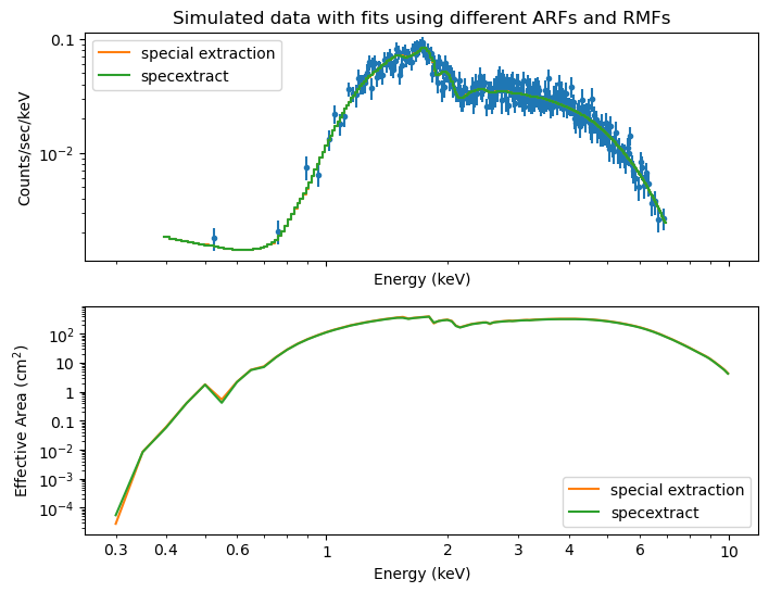
Powerlaw spectrum of an off-axis source
Same as above, but for an off-axis source on ACIS-I.
Input parameters
(some as above, but printed here again)
Model
| Component | Parameter | Thawed | Value | Min | Max | Units |
|---|---|---|---|---|---|---|
| xsphabs.a | nH | 1.0 | 0.0 | 1000000.0 | 10^22 atoms / cm^2 | |
| xspowerlaw.p | PhoIndex | 1.8 | -3.0 | 10.0 | ||
| norm | 0.001 | 0.0 | 1e+24 |
Fit with special extraction
confidence 1σ (68.2689%) bounds
| Parameter | Best-fit value | Lower Bound | Upper Bound |
|---|---|---|---|
| a1.nH | 0.981306 | -0.0537027 | 0.0555778 |
| p1.PhoIndex | 1.77587 | -0.0517193 | 0.0526568 |
| p1.norm | 0.000952562 | -6.49979e-05 | 7.13911e-05 |
Summary (3)
Fit with CIAO default extraction
confidence 1σ (68.2689%) bounds
| Parameter | Best-fit value | Lower Bound | Upper Bound |
|---|---|---|---|
| a2.nH | 0.979495 | -0.05391 | 0.0557851 |
| p2.PhoIndex | 1.77273 | -0.0516294 | 0.0528795 |
| p2.norm | 0.000971471 | -6.67038e-05 | 7.26692e-05 |
Summary (3)
For the off-axis simulation, the difference between the two extraction methods is smaller, probably because we are using the ACIS-I detector here.
Two thermal components on ACIS-I, on-axis
Same as above, but for a front-illuminated ACIS-I chip and using an input spectrum with two thermal components similar to a stellar corona.
Reading APEC data from 3.0.9
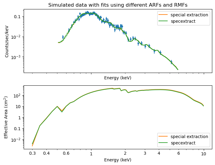
top: Simulated data and two model fits, assuming different ARFs and RMFs. “Special extraction” uses special qualifiers to match marx simulations, while “specextract” uses standard CIAO tools without any special qualifiers.
bottom: Shape of the ARFs used in the two extractions. Since the ARF is different, the model values are different when fitting to the same data (e.g. where the ARF is lower, the model flux has to be higher to match the data, leading to different slopes and normalizations in the two fits).
Input parameters
Model
| Component | Parameter | Thawed | Value | Min | Max | Units |
|---|---|---|---|---|---|---|
| xsvapec.apec1 | kT | 0.7 | 0.0808 | 68.447 | keV | |
| He | 1.0 | 0.0 | 1000.0 | |||
| C | 1.0 | 0.0 | 1000.0 | |||
| N | 1.0 | 0.0 | 1000.0 | |||
| O | 1.0 | 0.0 | 1000.0 | |||
| Ne | 2.0 | 0.0 | 1000.0 | |||
| Mg | 1.0 | 0.0 | 1000.0 | |||
| Al | 1.0 | 0.0 | 1000.0 | |||
| Si | 1.0 | 0.0 | 1000.0 | |||
| S | 1.0 | 0.0 | 1000.0 | |||
| Ar | 1.0 | 0.0 | 1000.0 | |||
| Ca | 1.0 | 0.0 | 1000.0 | |||
| Fe | 1.0 | 0.0 | 1000.0 | |||
| Ni | 1.0 | 0.0 | 1000.0 | |||
| Redshift | 0.0 | -0.999 | 10.0 | |||
| norm | 0.0002 | 0.0 | 1e+24 | |||
| xsvapec.apec2 | kT | 2.0 | 0.0808 | 68.447 | keV | |
| He | 1.0 | 0.0 | 1000.0 | |||
| C | 1.0 | 0.0 | 1000.0 | |||
| N | 1.0 | 0.0 | 1000.0 | |||
| O | 1.0 | 0.0 | 1000.0 | |||
| Ne | linked | 2.0 | ⇐ apec1.Ne | |||
| Mg | 1.0 | 0.0 | 1000.0 | |||
| Al | 1.0 | 0.0 | 1000.0 | |||
| Si | 1.0 | 0.0 | 1000.0 | |||
| S | 1.0 | 0.0 | 1000.0 | |||
| Ar | 1.0 | 0.0 | 1000.0 | |||
| Ca | 1.0 | 0.0 | 1000.0 | |||
| Fe | 1.0 | 0.0 | 1000.0 | |||
| Ni | 1.0 | 0.0 | 1000.0 | |||
| Redshift | 0.0 | -0.999 | 10.0 | |||
| norm | 0.0004 | 0.0 | 1e+24 | |||
Fit with special extraction
confidence 1σ (68.2689%) bounds
| Parameter | Best-fit value | Lower Bound | Upper Bound |
|---|---|---|---|
| apec1_1.kT | 0.700923 | -0.0405791 | 0.0369488 |
| apec1_1.Ne | 2.92372 | -1.1926 | 1.22549 |
| apec1_1.norm | 0.000202887 | -1.19405e-05 | 1.1852e-05 |
| apec2_1.kT | 2.01478 | -0.131887 | 0.153775 |
| apec2_1.norm | 0.000350393 | -2.31422e-05 | 2.35164e-05 |
Summary (3)
Fit with CIAO default extraction
confidence 1σ (68.2689%) bounds
| Parameter | Best-fit value | Lower Bound | Upper Bound |
|---|---|---|---|
| apec1_2.kT | 0.702725 | -0.0387937 | 0.0360131 |
| apec1_2.Ne | 2.93137 | -1.1744 | 1.19814 |
| apec1_2.norm | 0.000212816 | -1.22249e-05 | 1.21257e-05 |
| apec2_2.kT | 2.03402 | -0.137638 | 0.164865 |
| apec2_2.norm | 0.000367645 | -2.47575e-05 | 2.51193e-05 |
Summary (3)
Again we are looking at an ACIS-I simulation and the differences between the two extraction methods are smaller than for ACIS-S. While the Ne abundance is not well-constrained in this case, the fitted values are in general in agreement with the input values.
