Source shapes in MARX

marx offers different source shapes. Tests in this module exercise those sources (except SAOSAC, which is heavily used in the PSF tests already).

from utils import setup_marx
setup_marx()

Build-in geometric sources

This test exercises build-in |marx| sources with different geometric shapes. Most source types have parameters, and not all parameters are tested here. See source documentation for a detailed description of source parameters.

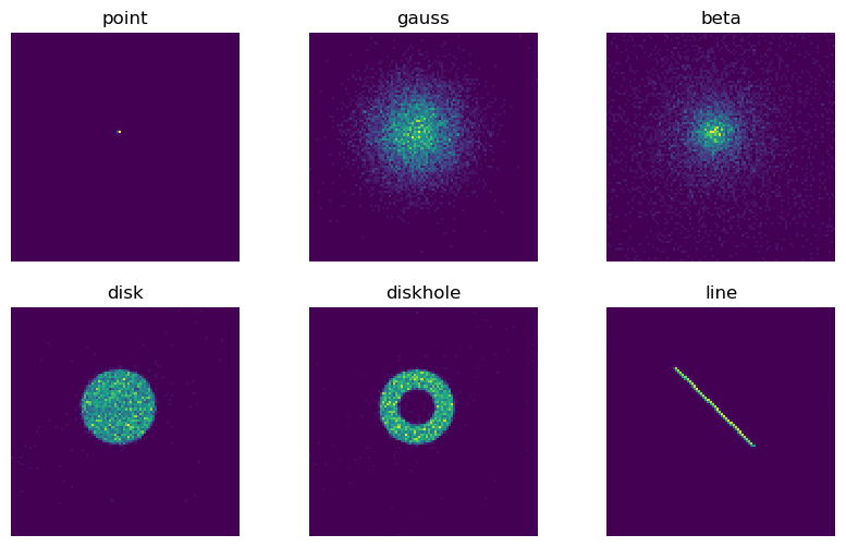
import subprocess

sources = [ {'OutputDir': 'point'}, # Default shape is POINT
            {'SourceType': 'GAUSS', 'S-GaussSigma': 20, 'OutputDir': 'gauss'},
            {'SourceType': 'BETA', 'S-BetaCoreRadius': 10,'S-BetaBeta': 0.6, 'OutputDir': 'beta'},
            {'SourceType': 'DISK', 'S-DiskTheta0': 0, 'S-DiskTheta1': 20, 'OutputDir': 'disk'},
            {'SourceType': 'DISK', 'S-DiskTheta0': 10, 'S-DiskTheta1': 20, 'OutputDir': 'diskhole'},
            {'SourceType': 'LINE', 'S-LinePhi': 45, 'S-LineTheta': 30, 'OutputDir': 'line'},
        ]
for src in sources:
    marxcall = ['marx GratingType=NONE'] + ['{0}={1}'.format(k, v) for k, v in src.items()]
    marxcall = ' '.join(marxcall)
    out = subprocess.run(marxcall, shell=True, capture_output=True)
    out2 = subprocess.run(f'marx2fits --pixadj=EDSER {src["OutputDir"]} {src["OutputDir"]}.fits', 
                             shell=True, capture_output=True)

from matplotlib import pyplot as plt
import pycrates

fig, axes = plt.subplots(2, 3, figsize=(10,6), subplot_kw={'aspect':'equal'})
for ax, src in zip(axes.flatten(), sources):
    evt = pycrates.read_file(f'{src["OutputDir"]}.fits')
    out = ax.hist2d(evt.get_column('X').values, evt.get_column('Y').values, 
                    bins=100, range=[[3900,4150], [4000,4250]])
    out = ax.set_title(src['OutputDir'])
    ax.set_axis_off()

Image as source

An image can be used as marx input. In this case, the intensity of the X-ray radiation on that sky is taken to be proportional to the value of the image at that point.

In this example we use Python to make a simple image as input, but one could use any fits image, e.g. a source observed in a different wavelength or the output of a simulation. In the Python code, we set up a 3-d box and fill it with an emitting shell. We then integrate along one dimension to obtain a collapsed image. Physically, this represents the thin shell of a supernova explosion.

import numpy as np
from astropy.wcs import WCS
from astropy.io import fits

# Actually to make this run faster, we'll do only one quadrant here
cube = np.zeros((201, 201, 201))
mg = np.mgrid[0: 201., 0:201, 0:201 ]
d = np.sqrt(mg[0, :, :, :]**2 + mg[1, :, :, :]**2 + mg[2, :, :, :]**2)
cube[(d > 160.) & (d < 170)] = 1
im = cube.sum(axis=0)
# Now rotate and put the four quarters together
image = np.zeros((401, 401))
image[:201, :201] = np.fliplr(np.flipud(im))
image[:201, 200:] = np.flipud(im)
image[200:, :201] = np.fliplr(im)
image[200:, 200:] = im

# Create a new WCS object.
w = WCS(naxis=2)
w.wcs.crpix = [100., 100.]
# Pixel size of our image shall be 1 arcsec
w.wcs.cdelt = [1. / 3600., 1. / 3600.]
w.wcs.ctype = ["RA---TAN", "DEC--TAN"]

# Now, write out the WCS object as a FITS header
header = w.to_header()

# header is an astropy.io.fits.Header object.  We can use it to create a new
# PrimaryHDU and write it to a file.
hdu = fits.PrimaryHDU(header=header, data=image)

# Save to FITS file
hdu.writeto('input_image.fits', overwrite=True)

out = subprocess.run('marx SourceType=IMAGE S-ImageFile=input_image.fits MinEnergy=1.9 MaxEnergy=1.9 GratingType=NONE OutputDir=image',
                      shell=True, capture_output=True)
out2 = subprocess.run(f'marx2fits --pixadj=EDSER image image.fits', 
                             shell=True, capture_output=True)

fig, axes = plt.subplots(1, 2, figsize=(10,6), subplot_kw={'aspect':'equal'})
input_image = pycrates.read_file('input_image.fits')
axes[0].imshow(image, origin='lower')
axes[0].set_title('input image')

evt = pycrates.read_file(f'image.fits')
out = axes[1].hist2d(evt.get_column('X').values, evt.get_column('Y').values, 
                    bins=100, range=[[3600,4600], [3600,4600]])
axes[1].set_title('Binned events from marx')
for ax in axes:
    ax.set_axis_off()

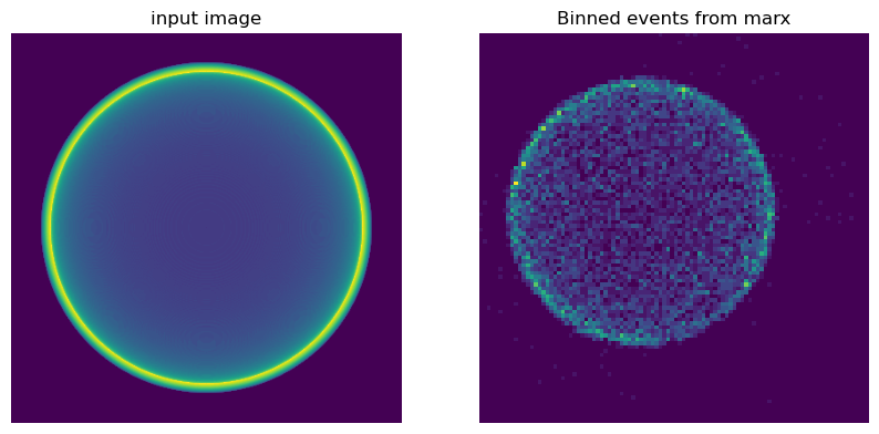
The left image shows the input image, the right image the binned events from marx using that image as source. Note that the apparent size of the images is different, since the scale is in pixels, not in Ra/Dec and the pixel size of the input image differs from the ACIS pixel size.

Using a RAYFILE source

marx is a Monte-Carlo code, thus the exact distribution of photons on the sky will be different every time the code is run. Sometimes it can be useful to generate a list of photons with position, time and energy from the source on the sky and then “observe” the exact same list with different instrument configurations so that any differences in the result are only due to the different configuration and not to random fluctuations in the source.

In this example, we look at a relatively large, diffuse emission region with a very soft spectrum (for simplicity we are using a flat spectrum). We compare simulations using ACIS-S and ACIS-I. ACIS-S has a better response to soft photons, but some parts of the source may not be in the field-of-view; ACIS-I is less efficient for soft photons, but has a larger field-of-view. For the simulation, we pick a date early in the Chandra mission, since the contamination layer on ACIS was still thin at the time. Today, neither ACIS-S nor ACIS-I would detect many photons from such a soft source.

out = subprocess.run('marx SourceType=GAUSS S-GaussSigma=300 MinEnergy=0.3 MaxEnergy=0.8 GratingType=NONE DumpToRayFile=yes ExposureTime=30000',
                      shell=True, capture_output=True)
for n in 'si':
    out = subprocess.run(f'marx SourceType=RAYFILE RayFile=marx.output OutputDir=acis{n} DetectorType=ACIS-{n.upper()} TStart=2005',
                         shell=True, capture_output=True)
    out2 = subprocess.run(f'marx2fits --pixadj=EXACT acis{n} acis{n}.fits', 
                             shell=True, capture_output=True)

from mpl_toolkits.axes_grid1 import ImageGrid
fig = plt.figure(figsize=(10,6))
grid = ImageGrid(
    fig, 111,  # similar to fig.add_subplot(142).
    nrows_ncols=(1, 2), axes_pad=0.4, label_mode="L", share_all=True,
    cbar_location="top", cbar_mode="each")
for ax, cax, src in zip(grid, grid.cbar_axes, ['aciss', 'acisi']):
    evt = pycrates.read_file(f'{src}.fits')
    im = ax.hist2d(evt.get_column('X').values, evt.get_column('Y').values, 
                    bins=50, range=[[3000,5000], [3000,5000]])
    out = ax.set_title('ACIS-' + src[-1].upper())
    cax.colorbar(im[-1])

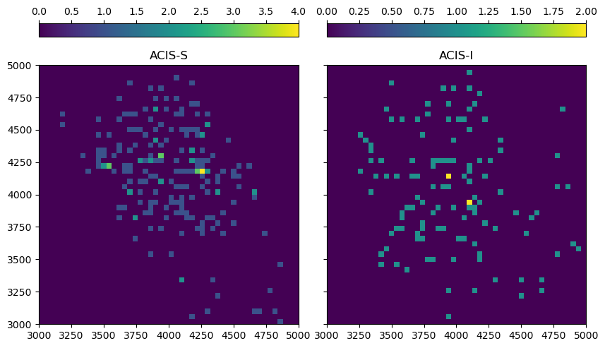
Both sources are generated from the same photon list. Sometimes the same pattern of photons can be seen in both images, but with a some events missing on ACIS-I due to the lower soft response, while others lie outside of the ACIS-S field-of-view.

Compiling a USER source

marx comes with several examples for user written sources in C. These can be compiled as shared objects and dynamically linked into marx at run time. To test this, we copy one of the source files from the installed marx version and compile it with gcc. This particular case is not very useful, because marx already has a point source with the same properties build-in. The purpose of this test is only to have a check that the dynamic linking works.

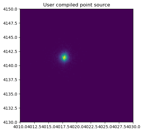
import os
import shutil

marxpath = os.path.dirname(shutil.which('marx'))
src = os.path.join(marxpath, '..',
                    'share', 'doc', 'marx', 'examples', 'user-source')
for f in ['point.c', 'user.h']:
    shutil.copy(os.path.join(src, f), f)
jdmath_h = os.path.join(marxpath, '..', 'include')
jdmath_a = os.path.join(marxpath, '..', 'lib', 'libjdmath.a')

out = subprocess.run(['gcc', '-I' + jdmath_h, jdmath_a,
                      '-shared', 'point.c', '-o', 'point.so'])

out = subprocess.run(f'marx SourceType=USER UserSourceFile=point.so GratingType=NONE OutputDir=userpoint',
                         shell=True, capture_output=True)
out2 = subprocess.run(f'marx2fits --pixadj=EDSER userpoint userpoint.fits', 
                             shell=True, capture_output=True)

fig, axes = plt.subplots(1, 1, figsize=(5, 5), subplot_kw={'aspect':'equal'})
evt = pycrates.read_file('userpoint.fits')
out = axes.hist2d(evt.get_column('X').values, evt.get_column('Y').values, 
                bins=100, range=[[4010,4030], [4130,4150]])
out = axes.set_title('User compiled point source')
#axes.set_axis_off()

The distribution of source is indeed a point source; it seems that we compiled and liked the user source file correctly.