Flight grade distribution

When an X-ray photon (or a highly energetic particle) hits the ACIS detector, it produces a charge cloud in the silicon of the chip. The size and the shape of the this charge cloud depends strongly on the energy of the event, the type of the event, and on the characteristics of the detector.

In many cases, the charge cloud is large enough to produce detectable signal in more than one pixel. This information is encoded in the “flight grade” (see the observatory guide for details). Flight grades are used to filter out background events by removing those grades where a large fraction of all detected events is due to particles and also in the sub-pixel event repositioning (EDSER). For example, grade “0” events have charge in one pixel only, and grade “2” indicates an event that has charge in two neighboring pixels. Most likely, the grade “0” event occurred close to the center of the pixel and the grade “2” event close to the boundary of the two pixels. Thus, simulating the right event grade distribution is a prerequisite to using any sub-pixel event repositioning algorithm on simulated data.

import os
import shutil

'''These environment parameters should be set before running the notebook,
but I didn't so, so I'm setting them here.'''

os.environ['PATH'] = '/Users/guenther/code/marx_installed/bin:' + os.environ['PATH']
os.environ['PFILES'] = os.path.dirname(shutil.which('marx')) + '/../share/marx/pfiles:' + os.environ['PFILES']

Grades on an ACIS-BI chip

This test compares the distribution of event grades between an observation of a young star observed on the back-illuminated S3 chip and the simulation. To avoid pile-up the observation used a sub-array read-out.

The grade distribution depends on the energy of the incoming photons. To get things exactly right, marx thus has to run with the source spectrum as an input spectrum. However, the grade distribution changes slowly with energy, so this only matters when grade distribution over a large range of energy are compared. Here, marx is run with a constant input spectrum and the comparison between simulation and observation is done in narrow energy bands only.

In this particular case, there is very little source signal above 2 keV, so the comparison is limited to low energies.

from contextlib import chdir
from matplotlib import pylab as plt

import pycrates
import ciao_contrib.runtool as rt
from ciao_contrib.cda.data import download_chandra_obsids

# Download data
out = download_chandra_obsids([15713], filetypes=['evt2', 'asol'])

asolfile = '15713/primary/pcadf15713_000N001_asol1.fits.gz'
evt2file = '15713/primary/acisf15713N003_evt2.fits.gz'

# Extract point source
rt.dmcopy(f"{evt2file}[sky=circle(12:09:02,-51:20:41,6)]", "obs.fits", clobber=True)

'''utility function that parses the fits header to set the marx parameters'''
from utils import marxpars_from_asol

pars = marxpars_from_asol(asolfile, evt2file)
pars['MinEnergy'] = 0.3
pars['MaxEnergy'] = 2.0

Here is the marx command that we will use to run the simulation, which matches the observation setup as closely as possible and runs the simulation in the energy band that we will analyze later on. This energy band is chosen, because that’s where the most photons in the observation are detected.

marxcall = ['marx'] + ['{0}={1}'.format(k, v) for k, v in pars.items()]
marxcall = ' '.join(marxcall)
marxcall

'marx RA_Nom=182.25561765981 Dec_Nom=-51.34945070544 Roll_Nom=33.971360241142 GratingType=NONE ExposureTime=10190.8068100214 DitherModel=FILE DitherFile=15713/primary/pcadf15713_000N001_asol1.fits TStart=508966864.84768 ACIS_Exposure_Time=0.7 SourceRA=182.259167 SourceDEC=-51.344667 DetectorType=ACIS-S DetOffsetX=0.0014449422646707344 DetOffsetZ=-0.007542945902798692 MinEnergy=0.3 MaxEnergy=2.0'

'''Currently, MARX can only be run from the command line. So we build
a command line call from the parameters dictionary and run it via
subprocess.call().'''
import subprocess
out = subprocess.run(marxcall, shell=True, capture_output=True)

out = subprocess.run('marx2fits --pixadj=EDSER point marxsim.fits', shell=True, 
                     capture_output=True)

'''Define plotting functions.

We will want to make the same matplotlib plot for different data sets,
so we define a function here that creates a 2x2 pie chart plot.'''
import numpy as np
def plotpie(ax, data, **plotargs):
    '''Bin up events data and display in pie chart'''
    counts = np.bincount(data)
    labels = np.arange(len(counts))
    ind = counts > 0
    ax.pie(counts[ind], labels=labels[ind],
           autopct='%2i%%', **plotargs)

def plot22(obs, sim, colname, energies=[[300, 1000], [1000, 2000]]):
    '''Place 2*2 piecharts on a figure.
    Parameters
    ----------
    obs : `pycrates.Crate`
        Observed events
    sim : `pycrates.Crate`
        Events simulated with MARX
    energies : list
        Two energy bands in eV defined as a list of lists.

    Returns
    -------
    fig : `matplotlib.figure.Figure`
        Figure with plot
    '''
    fig = plt.figure(figsize=(7, 7))
    for i, data in enumerate([obs, sim]):
        for j, en in enumerate(energies):
            ax = fig.add_subplot(2, 2, i * 2 + j + 1, aspect='equal')
            obssimlab = 'Obs' if i == 0 else 'MARX'
            energylab = '{0} - {1} eV'.format(en[0], en[1])
            ax.set_title('{0}: {1}'.format(obssimlab, energylab))
            energy = data.get_column('energy').values
            values = data.get_column(colname).values
            plotpie(ax, values[(energy > en[0]) & (energy < en[1])])
    return fig

obs = pycrates.read_file('obs.fits')
sim = pycrates.read_file('marxsim.fits')

fig = plot22(obs, sim, 'grade')

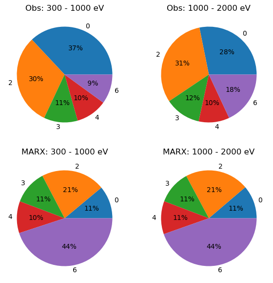
These pie charts show the distribution of grades in ASCA nomenclature (0-6) in two different energy bands.

fig = plot22(obs, sim, 'fltgrade')

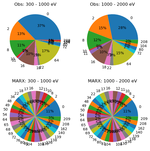
Same as the above, but using the more detailed Chandra flight grade numbers.

Both plots clearly show that MARX does not do a good job either at reproducing the distribution of grades in general, nor in reproducing the energy dependence.

Grades on an ACIS-FI chip

This compares the grade distribution for a front-illuminated (FI) chip.

'''We repeat the code from above changing just the ObsID, source coordinates, and energy range.'''
out = download_chandra_obsids([4496], filetypes=['evt2', 'asol'])

asolfile = '4496/primary/pcadf04496_000N001_asol1.fits.gz'
evt2file = '4496/primary/acisf04496N004_evt2.fits.gz'

rt.dmcopy(f"{evt2file}[sky=circle(11:11:53.3,-61:18:46,4)]", "obs.fits", clobber=True)

'''Run in energy band, match observational setup'''
pars = marxpars_from_asol(asolfile, evt2file)
pars['MinEnergy'] = 2.0
pars['MaxEnergy'] = 4.0

marxcall = ['marx'] + ['{0}={1}'.format(k, v) for k, v in pars.items()]
out = subprocess.run(' '.join(marxcall), shell=True, capture_output=True)

out = subprocess.run('marx2fits --pixadj=EDSER point marxsim.fits', shell=True,
                     capture_output=True)

obs = pycrates.read_file('obs.fits')
sim = pycrates.read_file('marxsim.fits')

fig = plot22(obs, sim, 'grade')

fig = plot22(obs, sim, 'fltgrade')

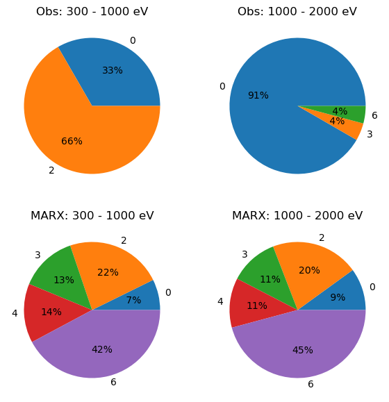
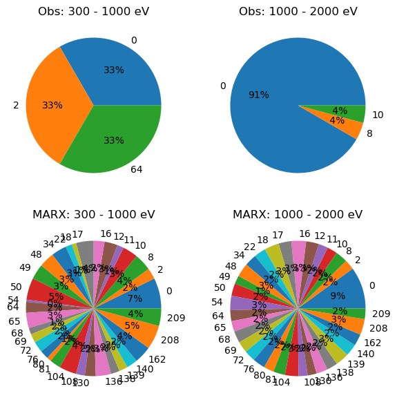
Again, both plots clearly show that MARX does not do a good job either at reproducing the distribution of grades in general, nor in reproducing the energy dependence.’’’