from utils import setup_marx
setup_marx()

Coordinates on the sky and the chip

In every marx simulation, one or more sources are placed at some sky position. marx simulates photons coming from that position, traces them through the mirror and gratings and finally places them on the chip. With a known aspect solution, chip coordinates can then be transformed back to sky coordinates. In general, this will not recover the exact sky position where a photon started out. A big part of that is scatter in the mirrors, which blurs the image. However, with a large number of photons, we can fit the average position which should be close to the real sky position.

In real observations, other factors contribute, such as the finite resolution of the detectors (marx usually takes that into account, but it can be switched off through the --pixadj="EXACT" switch in marx2fits) and the uncertainty of the aspect solution.

Within a single observation, positions will be less certain for fainter sources (due to Poisson statistics) and for sources at a larger off-axis angles (due to the larger PSF).

Chandra Orion Ultradeep project

The Orion Nebula Cluster (ONC) is a dense star forming region with about 1600 X-ray sources observed in the COUP survey by Getman et al (2005). We simulate this field with marx and then run a source detection to check how well we recover the input coordinates. This will depend on the number of counts detected and the position in the field. To simplify the simulation input, we assume that all sources have flat lightcurves and are monoenergetic at the observed mean energy (the energy matters because the effective area is energy dependent and so is the PSF). We write a short C code that reads an input coordinate list and generates the photons in this manner.

from ciao_contrib.cda.data import download_chandra_obsids

out = download_chandra_obsids([3744], filetypes=['asol', 'evt2'])

asolfile = '3744/primary/pcadf03744_000N001_asol1.fits.gz'
evt2file = '3744/primary/acisf03744N004_evt2.fits.gz'

'''Make input coordinate table

- Coordinates are relative to pointing direction in arcmin
- weight is a measure for the fraction on photons coming from that source, i.e. a linear luminosity
- For the source spectrum, we just take a mono-energetic source with the average energy.
'''
import os
from astropy.table import Table
from astropy.io import fits

asol = fits.getheader(asolfile, 1)
coup = Table.read(os.path.join('data', 'COUP.tsv'), format='ascii.fast_tab')
tab = Table()
tab['RA'] = (coup['RAJ2000'] - asol['RA_NOM']) * 60
tab['DEC'] = (coup['DEJ2000'] - asol['DEC_NOM']) * 60
tab['weight'] = 10**(coup['Lt'] - 27)
tab['energy'] = coup['<E>']
tab.write('coup.marxin', format='ascii.no_header', overwrite=True)

'''C code for a grid of sources.

(``user.h`` and ``jdmath.h`` are shipped with marx.)'''
ccode=r'''
#include <stdio.h>
#include <stdlib.h>
#include <jdmath.h>
#include "user.h"

/* This user source implements many point sources via a file that
 * specifies the source positions and energies.  The current implementation
 * assumes the format:
 *  RA  Dec weight energy
 * Here RA, Dec specify the source position, weight specifies the strength
 * of the source in relation to the others.
 */
typedef struct
{
   double cosx, cosy, cosz;
   double weight;
   double energy;
}
Point_Source_Type;

static unsigned int Num_Points;
static Point_Source_Type *Point_Sources;
static unsigned int Max_Num_Points;

static char *do_realloc (char *p, unsigned int len)
{
   if (p == NULL)
     p = malloc (len);
   else
     p = realloc (p, len);

   if (p == NULL)
     fprintf (stderr, "Not enough memory\n");

   return p;
}

static void free_sources (void)
{
   if (Point_Sources == NULL)
     return;

   free ((char *) Point_Sources);
   Point_Sources = NULL;
}

static int add_source (double ra, double dec, double weight, double energy)
{
   Point_Source_Type *p;
   double cosx, cosy, cosz;

   /* Convert to God's units from arc-min */
   ra = ra * (PI/(180.0 * 60.0));
   dec = dec * (PI/(180.0 * 60.0));

   if (Max_Num_Points == Num_Points)
     {
        Max_Num_Points += 32;
        p = (Point_Source_Type *)do_realloc ((char *)Point_Sources, Max_Num_Points * sizeof (Point_Source_Type));
        if (p == NULL)
          {
             free_sources ();
             return -1;
          }
        Point_Sources = p;
     }

   p = Point_Sources + Num_Points;
   /* Note the the minus sign is to generate a vector pointing from the
    * source to the origin
    */
   p->cosx = -cos (dec) * cos (ra);
   p->cosy = -cos (dec) * sin(ra);
   p->cosz = -sin (dec);

   p->weight = weight;
   p->energy = energy;
   Num_Points += 1;

   return 0;
}

static void normalize_sources (void)
{
   double total;
   unsigned int i;

   total = 0;
   for (i = 0; i < Num_Points; i++)
     {
	Point_Sources[i].weight += total;
	total = Point_Sources[i].weight;
     }

   for (i = 0; i < Num_Points; i++)
     Point_Sources[i].weight /= total;

   /* Make sure no round-off error affects the weight of the last point */
   Point_Sources[Num_Points - 1].weight = 1.0;
}

int user_open_source (char **argv, int argc, double area,
		      double cosx, double cosy, double cosz)
{
   FILE *fp;
   char line[1024];
   char *file;
   unsigned int linenum;

   file = argv[0];
   if (file == NULL)
     {
	fprintf (stderr, "UserSource Model requires FILE as argument\n");
	return -1;
     }

   fp = fopen (file, "r");
   if (fp == NULL)
     {
	fprintf (stderr, "Unable to open %s\n", file);
	return -1;
     }

   linenum = 0;
   while (NULL != fgets (line, sizeof (line), fp))
     {
	double ra, dec, weight, energy;

	linenum++;
	if (4 != sscanf (line, "%lf %lf %lf %lf", &ra, &dec, &weight, &energy))
	  continue;

	if (weight <= 0.0)
	  {
	     fprintf (stderr, "weight on line %d of %s must be positive\n",
		      linenum, file);
	     free_sources ();
	     return -1;
	  }

	if (-1 == add_source (ra, dec, weight, energy))
	  {
	     fclose (fp);
	     return -1;
	  }
     }

   fclose (fp);
   if (Num_Points == 0)
     {
	fprintf (stderr, "%s contains no sources\n", file);
	return -1;
     }

   normalize_sources ();
   return 0;
}

void user_close_source (void)
{
   free_sources ();
}


int user_create_ray (double *delta_t, double *energy,
		     double *cosx, double *cosy, double *cosz)
{
   double r;
   Point_Source_Type *p;

   p = Point_Sources;

   r = JDMrandom ();
   while (r > p->weight)
     p++;

   *delta_t = -1.0;
   *energy = p->energy;
   *cosx = p->cosx;
   *cosy = p->cosy;
   *cosz = p->cosz;

   return 0;
}

int main (int a, char **b)
{
   (void) a;
   (void) b;
   return 1;
}
'''

with open('pnts.c', 'w') as f:
    f.write(ccode)

import shutil
import subprocess

marxpath = os.path.dirname(shutil.which('marx'))
src = os.path.join(marxpath, '..',
                    'share', 'doc', 'marx', 'examples', 'user-source')
shutil.copy(os.path.join(src, 'user.h'), 'user.h')
jdmath_h = os.path.join(marxpath, '..', 'include')
jdmath_a = os.path.join(marxpath, '..', 'lib', 'libjdmath.a')

out = subprocess.run(['gcc', '-I' + jdmath_h, jdmath_a,
                      '-shared', 'pnts.c', '-o', 'pnts.so'])

from utils import marxpars_from_asol
pars = marxpars_from_asol(asolfile, evt2file)
pars['OutputDir'] = 'COUP'
pars['SourceType'] = 'USER'
pars['UserSourceFile'] = 'pnts.so'
pars['UserSourceArgs'] = 'coup.marxin'
# We could try to rigorously determine the total flux of the field
# but here we just pick a number that will give us a good number of photons.
pars['SourceFlux'] = 0.03

marxcall = ['marx'] + ['{0}={1}'.format(k, v) for k, v in pars.items()]
marxcall = ' '.join(marxcall)

'''Currently, MARX can only be run from the command line. So we build
a command line call from the parameters dictionary and run it via
subprocess.call().'''

out = subprocess.run(marxcall, shell=True, capture_output=True)
out2 = subprocess.run('marx2fits --pixadj=EDSER COUP COUP.fits', shell=True, capture_output=True)

In the observation, the brightest sources are piled-up. We don’t bother simulating this here, so for the visualization we just set the scaling limits to bring out the fainter details and ignore the bright peaks.

from astropy.visualization import simple_norm
import numpy as np
from mpl_toolkits.axes_grid1 import ImageGrid
import matplotlib.pyplot as plt
import pycrates

fig = plt.figure(figsize=(12,6))
grid = ImageGrid(
    fig, 111,  # similar to fig.add_subplot(142).
    nrows_ncols=(1, 2), axes_pad=0.4, label_mode="L", share_all=True,
    cbar_location="top", cbar_mode="single")
for ax, cax, src, title in zip(grid, grid.cbar_axes, 
                               [evt2file, 'COUP.fits'], 
                               ['Observation', 'MARX Simulation']):
    evt = pycrates.read_file(src)
    hist= np.histogram2d(evt.get_column('X').values, evt.get_column('Y').values, 
                    bins=600, range=[[3900,4500], [3900,4500]])
    norm = simple_norm(hist[0], 'log', vmax=300)
    im = ax.imshow(hist[0].T, origin='lower', extent=[3900,4500,3900,4500], norm=norm)
    out = ax.set_title(title)
    cbar = cax.colorbar(im)
    cbar.set_label('Counts per bin')

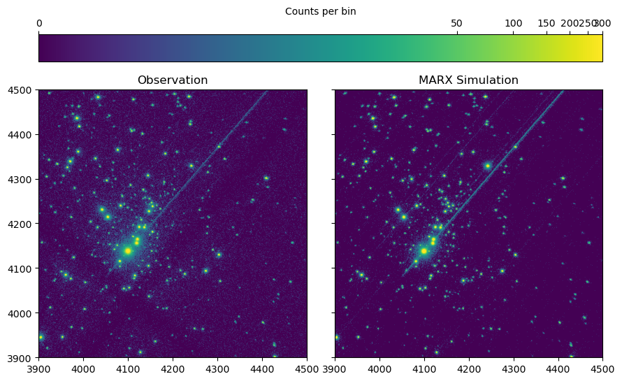
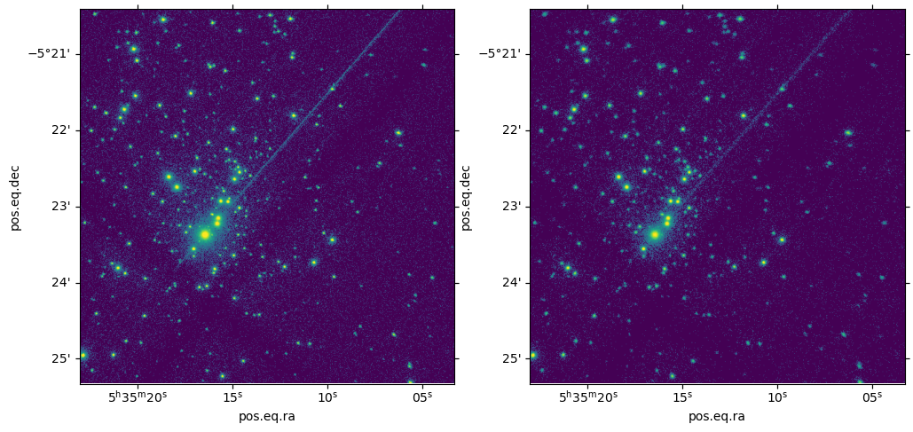
Image of the observed data (left) and simulation (right). The diagonal line from the center to the top right is the read-out streak from $\theta^1$ Ori C.

from ciao_contrib import runtool as rt

rt.dmcopy("COUP.fits[EVENTS][bin x=2500:5500:2,y=2500:5500:2]", "im.fits", option="image",
           clobber=True)
rt.mkpsfmap("im.fits", "psf.map", energy=1.4, ecf=0.5, clobber=True)
rt.celldetect("im.fits", "src.fits", psffile="psf.map", clobber=True)

from astropy.coordinates import SkyCoord
from astropy.io import fits
src = Table.read('src.fits')

src_co = SkyCoord(src['RA'], src['DEC'], unit='deg')
srcin_co = SkyCoord(coup['RAJ2000'], coup['DEJ2000'], unit='deg')
idx, d2d, d3d = src_co.match_to_catalog_sky(srcin_co)

asol = fits.getheader(asolfile, 1)
cen = SkyCoord(asol['RA_NOM'], asol['DEC_NOM'], unit='deg')
d = cen.separation(src_co).arcsec

fig = plt.figure()
ax1 = plt.subplot(111)
scat1 = ax1.scatter(d, d2d.arcsec, c=np.log10(src['NET_COUNTS']), lw=1)
ax1.set_xlabel('distance from aimpoint [arcsec]')
ax1.set_ylabel('coordinate error [arcsec]')
ax1.set_xlim([0, 350])
ax1.set_ylim([0, 2])
cbar1 = fig.colorbar(scat1, ax=ax1)
cbar1.set_label('log(net counts per source)')

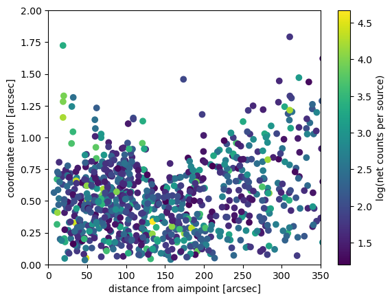
Apart from a clump close to the aimpoint (where sources in the ONC are so close to each other that they can easily be confused), the distribution of coordinate errors spreads out with increasing distance, i.e. size of the PSF.

Simulations with an IMAGE source

The SourceType=IMAGE in marx is a strange beast that behaves in ways that users might find surprising. When using this source type, marx will read in an image file and use the pixel values as relative probabilities for generating photons across the image.

Marx will read the WCS in the image header, but only use the absolute value for the pixel size, not the orientation or position. The center of the image is always supposed to be at the nominal pointing position and the image x/y axes are always aligned with the sky coordinate system in marx.

# Turn the downloaded event file into an image
from ciao_contrib import runtool as rt
rt.dmcopy.punlearn()
rt.dmcopy(evt2file + '[bin x=3900:4500:1,y=3900:4500:1]', '3744_image.fits', clobber=True)

# Are using astropy for the coordinate transforms, just because I know it better and can type it faster
# than the equivalent packages that are part of CIAO
from astropy.wcs import WCS
from astropy.io import fits

# Fortunately, the chandra X/Y axes are already aligned with the axes that marx uses,
# so no image rotation is needed here.
with fits.open('3744_image.fits') as hdus:
    wcs = WCS(hdus[0].header, fix=False)
    shape = hdus[0].data.shape
center = wcs.pixel_to_world(shape[0]/2, shape[1]/2)

'''MARX simulation with an IMAGE source 
'''
pars['SourceFlux'] = 0.003 # speed up during experimentation

pars['SourceType'] = 'IMAGE'
pars['S-ImageFile'] = '3744_image.fits'
pars['OutputDir'] = 'COUP_image'
pars['SourceRA'] = center.ra.deg
pars['SourceDEC'] = center.dec.deg
pars['DitherModel'] = 'INTERNAL'

marxcall = ['marx'] + ['{0}={1}'.format(k, v) for k, v in pars.items()]
marxcall = ' '.join(marxcall)
out = subprocess.run(marxcall, shell=True, capture_output=True)
out2 = subprocess.run('marx2fits --pixadj=EDSER COUP_image COUP_image_evt2.fits',
                      shell=True, capture_output=True)

# Let's turn the simulated data into an image, too, to make it easier to 
# display in WCS instead of in detector coordinates
rt.dmcopy('COUP_image_evt2.fits[bin x=3900:4500:1,y=3900:4500:1]', 'COUP_image.fits', clobber=True)

fig = plt.figure(figsize=(12,6))
for i, f in enumerate(['3744_image.fits', 'COUP_image.fits'], start=1):
    with fits.open(f) as hdus:
        wcs = WCS(hdus[0].header, fix=False)
        data = hdus[0].data
    norm = simple_norm(data, 'log', vmax=300)
    ax = fig.add_subplot(1, 2, i, projection=wcs)
    ax.imshow(data, norm=norm, origin='lower')

WARNING: FITSFixedWarning: RADECSYS= 'ICRS ' / WCS system 
the RADECSYS keyword is deprecated, use RADESYSa. [astropy.wcs.wcs]

Regular Grid (ACIS)

In this example we place a radial grid of sources on the sky. Each source emits an equal number of photons (exactly, no Poisson statistics) so that we can compare the accuracy of the position we recover. Note that the detected number of photons will be smaller for off-axis photons because of vignetting!

ccode='''
#include <stdio.h>
#include <math.h>
#include "user.h"

static double Source_CosX;
static double Source_CosY;
static double Source_CosZ;

int user_open_source (char **argv, int argc, double area,
		      double cosx, double cosy, double cosz)
{
   return 0;
}

void user_close_source (void)
{
}

static double To_Radians = (M_PI / 180.0 / 3600.0);
#define ARC_SECONDS_PER_CELL 50
#define ANGULAR_STEPS 16

int user_create_ray (double *delta_t, double *energy,
		     double *cosx, double *cosy, double *cosz)
{
   static int last_i = 0;
   static int last_j = 0;
   double theta, phi;
   double cos_theta, sin_theta;

   if (last_j == ANGULAR_STEPS){
        last_j = 0;
        last_i++;
   }
   if (last_i == 20) last_i = 0;

   theta = To_Radians * last_i * ARC_SECONDS_PER_CELL;
   phi = (10. /180 * M_PI) + last_j * 2 * M_PI / ANGULAR_STEPS;

   sin_theta = sin(theta);

   *cosx = -cos (theta);
   *cosy = sin_theta * cos (phi);
   *cosz = sin_theta * sin (phi);

   *delta_t = -1.0;
   *energy = -1.0;

   if (last_i ==0){
     last_i++;
        }
   else {
     last_j++;
        }

   return 0;
}

int main (int a, char **b)
{
   (void) a;
   (void) b;
   return 1;
}'''
with open('radialgrid.c', 'w') as f:
    f.write(ccode)

out = subprocess.run(['gcc', '-lm',
                      '-shared', 'radialgrid.c', '-o', 'radialgrid.so'])

pars = {'SourceType': 'USER', 'OutputDir': 'points',
        'GratingType': 'NONE','SourceRA': 90., 'SourceDEC': 0.,
        'RA_Nom': 90., 'Dec_Nom': 0, 'Roll_Nom': 0,
        'DetectorType': 'ACIS-I',
        'UserSourceFile': 'radialgrid.so',
        'NumRays': -100000, 'ExposureTime': 0}
marxcall = ['marx'] + ['{0}={1}'.format(k, v) for k, v in pars.items()]
marxcall = ' '.join(marxcall)

'''Currently, MARX can only be run from the command line. So we build
a command line call from the parameters dictionary and run it via
subprocess.call().'''

out = subprocess.run(marxcall, shell=True, capture_output=True)
out2 = subprocess.run('marx2fits --pixadj=EDSER points points.fits', shell=True, capture_output=True)

fig, ax = plt.subplots(figsize=(6,6))

evt = pycrates.read_file('points.fits')
hist= np.histogram2d(evt.get_column('X').values, evt.get_column('Y').values, 
                bins=600, range=[[4097-1200,4097+1200], [4097-1200,4097+1200]])
norm = simple_norm(hist[0], 'log') #, vmax=300)
im = ax.imshow(hist[0].T, origin='lower', extent=[4097-1200,4097+1200,4097-1200,4097+1200], norm=norm)
cbar = plt.colorbar(im)
cbar.set_label('Counts per bin')

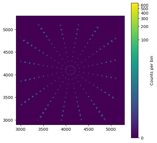
Image of the simulation. The size of the PSF increases further away from the aimpoint.

rt.dmcopy("points.fits[EVENTS][bin x=3000:5100:1,y=3000:5100:1]", "im.fits", option="image",
           clobber=True)
rt.mkpsfmap("im.fits", "psf.map", energy=1.4, ecf=0.5, clobber=True)
rt.celldetect("im.fits", "src.fits", psffile="psf.map", clobber=True)

src = Table.read('src.fits')
# Find distance from input position.
src['RA_INPUT'] = src['RA'] - (src['RA'] // (360./16.)) * (360./16.) - 10.
# Problem: Might expect source at 1.0,
# but measure at 0.99. In this case distance to next lower source
# is 0.99. Thus shift input by 0.005 (about 50 arcsec / 2)
# before integer devision
src['DEC_INPUT'] = src['DEC'] - ((0.005 + src['DEC']) // (50./3600.)) * (50./3600.)

cen = SkyCoord(90., 0, unit='deg')
det = SkyCoord(src['RA'], src['DEC'], unit='deg')
d = cen.separation(det).arcsec
d_err = np.mod(d + 10, 50.) - 10

ang = cen.position_angle(det).degree
# Subtract offset that we placed in the C code to avoid 0./360. ambiguity
# Step width is 360./16 = 22.5 deg
# Offset is 10 deg. Complement we find here is 12.5 deg.
ang = ang - 12.5

ang_err = np.mod(ang + 2, 360. / 16.) - 2
ind = d > 10

fig, (ax1, ax2) = plt.subplots(1, 2, figsize=(8, 4))
scat1 = ax1.scatter(d, d_err, c=src['NET_COUNTS'], lw=1)
ax1.set_xlabel('distance [arcsec]')
ax1.set_ylabel('distance error [arcsec]')
ax1.set_xlim([-10, 620])
ax1.set_ylim([-1, 0.5])
scat2 = ax2.scatter(ang, ang_err, c=src['NET_COUNTS'], lw=1)
ax2.set_xlabel('pos ang [deg]')
ax2.set_ylabel('pos ang error [deg]')
ax2.set_xlim([-5, 350])
ax2.set_ylim([-0.3, 0.3])
cbar2 = fig.colorbar(scat2, ax=ax2)
cbar2.set_label('net counts per source')
fig.tight_layout()

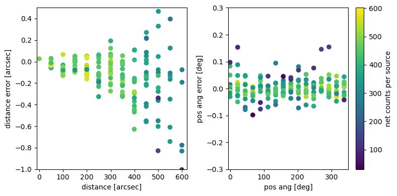
left: The error in the position (measured radially to the optical axis) increases with the distance to the optical axis. One part of this is just that the effective area and thus the number of counts decreases. There is also a systematic trend where sources at larger off-axis angle are systematically fitted too close to the center. Further investigation is necessary to check if this is a problem of marx or the CIAO tool celldetect. In any case, the typical offset is below 0.2 arcsec, which is less than half a pixel in ACIS. right: Difference in position angle between input and fit.

The input position is typically recovered to much better than one pixel for sources with a few hundred counts. There is a small systematic trend that needs to be studied further.

Regular grid (HRC)

Same as above, but with HRC-I as a detector.

The field-of-view for the HRC-I is larger for than for ACIS-I, but the PSF becomes very large at large off-axis angles and thus the positional uncertainty will be so large that a comparison to marx is no longer helpful to test the accuracy of the marx simulations.

pars['DetectorType'] = 'HRC-I'
marxcall = ['marx'] + ['{0}={1}'.format(k, v) for k, v in pars.items()]
marxcall = ' '.join(marxcall)

out = subprocess.run(marxcall, shell=True, capture_output=True)
out2 = subprocess.run('marx2fits --pixadj=EDSER points points.fits', shell=True, capture_output=True)

fig, ax = plt.subplots(figsize=(6,6))

evt = pycrates.read_file('points.fits')
hist= np.histogram2d(evt.get_column('X').values, evt.get_column('Y').values, 
                bins=600, range=[[16292-4000,16292+4000], [16392-4000,16392+4000]])
norm = simple_norm(hist[0], 'log') #, vmax=300)
im = ax.imshow(hist[0].T, origin='lower', extent=[16292-4000,16292+4000,16392-4000,16392+4000], norm=norm)
cbar = plt.colorbar(im)
cbar.set_label('Counts per bin')

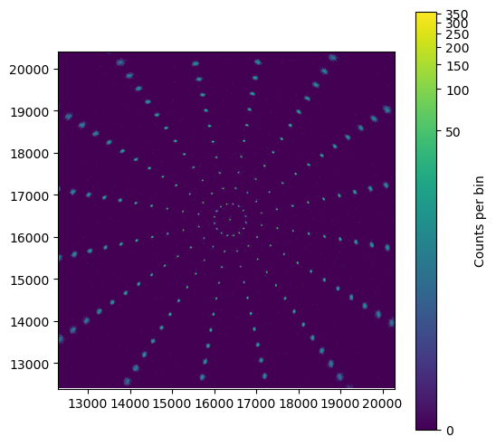
Image of the simulation. The size of the PSF increases further away from the aimpoint.

rt.dmcopy("points.fits[EVENTS][bin x=8500:24500:2,y=8500:24500:2]", "im.fits", option="image",
           clobber=True)
rt.mkpsfmap("im.fits", "psf.map", energy=1.4, ecf=0.5, clobber=True)
rt.celldetect("im.fits", "src.fits", psffile="psf.map", clobber=True)

src = Table.read('src.fits')
src['RA_INPUT'] = src['RA'] - (src['RA'] // (360./16.)) * (360./16.) - 10.
src['DEC_INPUT'] = src['DEC'] - ((0.005 + src['DEC']) // (50./3600.)) * (50./3600.)

cen = SkyCoord(90., 0, unit='deg')
det = SkyCoord(src['RA'], src['DEC'], unit='deg')
d = cen.separation(det).arcsec
d_err = np.mod(d + 10, 50.) - 10

ang = cen.position_angle(det).degree
# Subtract offset that we placed in the C code to avoid 0./360. ambiguity
# Step width is 360./16 = 22.5 deg
# Offset is 10 deg. Complement we find here is 12.5 deg.
ang = ang - 12.5

ang_err = np.mod(ang + 2, 360. / 16.) - 2
ind = d > 10

fig, (ax1, ax2) = plt.subplots(1, 2, figsize=(8, 4))
scat1 = ax1.scatter(d, d_err, c=src['NET_COUNTS'], lw=1)
ax1.set_xlabel('distance [arcsec]')
ax1.set_ylabel('distance error [arcsec]')
ax1.set_xlim([-10, 620])
ax1.set_ylim([-1, 0.5])
scat2 = ax2.scatter(ang, ang_err, c=src['NET_COUNTS'], lw=1)
ax2.set_xlabel('pos ang [deg]')
ax2.set_ylabel('pos ang error [deg]')
ax2.set_xlim([-5, 350])
ax2.set_ylim([-0.3, 0.3])
cbar2 = fig.colorbar(scat2, ax=ax2)
cbar2.set_label('net counts per source')
fig.tight_layout()

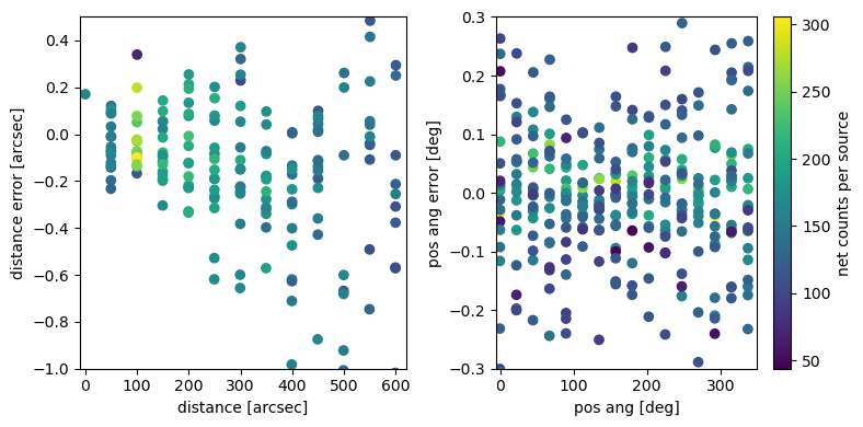
See previous example. The same trends are visible with a slightly larger scatter.

In the central few arcmin the input position is typically recovered to better than 0.2 pixels for sources with a few hundred counts.