from utils import setup_marx, setup_saotrace
setup_marx()
trace_nest = setup_saotrace()
Wings of the Chandra PSF
The Chandra PSF falls in two regimes: The shape of the core is set by quasi-specular reflection from low-frequency surface errors. This component is strongly peaked and dominates in the innermost few arcseconds (for and on-axis source). The out part of the PSF has the shape of a powerlaw with a spectral index close to two and is caused by micro-roughness on the mirror surfaces. The Proposer’s Observatory Guide and a memo by T.J. Gaetz discuss this in a lot more detail. The memo is based on a very detailed analysis of a deep Her-X1 observation. In this test we replicate that observation in marx and SAOTrace simulations.
In the memo, T.J. Gaetz goes to great lengths to separate the effect of the intrinsic Chandra PSF on the data from other influences such as the ACIS contamination. When we compare data and marx simulation below, we chose a somewhat simpler approach. We perform steps to mitigate the impact of other astrophysical sources (which are not part of the marx simulation) and background (which is not part of the marx simulation). On the other hand, we just compare the observed count rates with no correction for the ACIS contamination, dithering near chip edges etc. because those effects are included in both the observed and the simulated data.
Read the code for this test to see all details of the data extraction, but here are the most important points:
The source is heavily piled-up, thus the source spectrum is taken from the read-out streak.
Because of pile-up in the data, all fitting is restricted to radii above 15 arcsec.
from astropy.coordinates import SkyCoord
from astropy.io import fits
import numpy as np
import ciao_contrib.runtool as rt
from ciao_contrib.cda.data import download_chandra_obsids
from coords.chandra import cel_to_chandra
from utils import marxpars_from_asol, write_spectrum_from_fluxcorrection
out = download_chandra_obsids([3662])
asolfile = '3662/primary/pcadf03662_000N001_asol1.fits.gz'
evt2file = '3662/primary/acisf03662N004_evt2.fits.gz'
'''Source is heavily piled-up so we extract the source spectrum from the read-out streak.'''
source_reg = 'rotbox(3922.6168,3556.9146,12,512,332.71498)'
'''The analysis makes narrow band count rate images.
Bands are defined here. If they are too wide, then the effective area and spectrum
within one band cannot be taken as constant any longer, but if they are too narrow
the test will need a very long time to run.
'''
energy_bins = np.array([.4, .5, .6, .7, .9, 1., 1.2, 1.4, 1.6, 1.8, 2.0, 2.2, 2.4, 2.6, 2.8, 3.,
3.5, 4., 4.5, 5., 5.5, 6., 6.5, 7., 7.5, 8.])
mid_bins = 0.5 * (energy_bins[:-1] + energy_bins[1:])
sky_coos = SkyCoord.from_name('Her X-1')
coos = cel_to_chandra(fits.getheader(evt2file, 1), sky_coos.ra.degree, sky_coos.dec.degree)
x = coos['x'][0]
y = coos['y'][0]
write_spectrum_from_fluxcorrection(asolfile, evt2file, x, y, source_reg,
# Rough estimate of normalization
# Read-out streak region is 512 pix long
0.00004*512/3.2)
WARNING: UnitsWarning: 'channel' did not parse as fits unit: At col 0, Unit 'channel' not supported by the FITS standard. If this is meant to be a custom unit, define it with 'u.def_unit'. To have it recognized inside a file reader or other code, enable it with 'u.add_enabled_units'. For details, see https://docs.astropy.org/en/latest/units/combining_and_defining.html [astropy.units.core]
import subprocess
pars = marxpars_from_asol(asolfile, evt2file)
pars['SpectrumType'] = 'FILE'
pars['SpectrumFile'] = 'input_spec_marx.tbl'
pars['OutputDir'] = 'marx_only'
pars['SourceFlux'] = -1
marxcall = ['marx'] + ['{0}={1}'.format(k, v) for k, v in pars.items()]
marxcall = ' '.join(marxcall)
out = subprocess.run(marxcall, shell=True, capture_output=True)
asolh = fits.getheader(asolfile, 1)
evth = fits.getheader(evt2file, 1)
lua_text = f'''
ra_pnt = {asolh['RA_NOM']}
dec_pnt = {asolh['DEC_NOM']}
roll_pnt = {asolh['ROLL_NOM']}
dither_asol_chandra{{ file = "{asolfile}",
ra = ra_pnt, dec = dec_pnt, roll = roll_pnt }}
point{{ position = {{ ra = {evth['RA_TARG']},
dec = {evth['DEC_TARG']},
ra_aimpt = ra_pnt,
dec_aimpt = dec_pnt,
}},
spectrum = {{ {{ file = "input_spec_saotrace.rdb",
units = "photons/s/cm2",
scale = 1,
format = "rdb",
emin = "ENERG_LO",
emax = "ENERG_HI",
flux = "flux"}} }}
}}
'''
with open('saotrace_source.lua', 'w') as f:
f.write(lua_text)
'''
CXO time numbers are large and round-off error can appear
which make SAOTrace fail.
Therefore, shorten all times by about 0.01 sec to make sure.
'''
limit = asolh['TSTOP'] - asolh['TSTART']
limit = limit - 0.02
subprocess.run(trace_nest +
f' tag=saotrace srcpars=saotrace_source.lua tstart={asolh["TSTART"] + 0.01} limit={limit} limit_type=sec',
shell=True)
WARNING: image platform (linux/amd64) does not match the expected platform (linux/arm64)
CompletedProcess(args='/Users/guenther/code/saotrace-2.0.6.1/run-saotrace trace-nest tag=saotrace srcpars=saotrace_source.lua tstart=141954141.92872 limit=51150.81333998919 limit_type=sec', returncode=0)
pars['OutputDir'] = 'marx_saotrace'
pars['SourceType'] = 'SAOSAC'
pars['SAOSACFile'] = 'saotrace.fits'
marxcall = ['marx'] + ['{0}={1}'.format(k, v) for k, v in pars.items()]
marxcall = ' '.join(marxcall)
out = subprocess.run(marxcall, shell=True, capture_output=True)
out = subprocess.run('marx2fits --pixadj=EDSER marx_only marx_only.fits', shell=True,
capture_output=True)
out2 = subprocess.run('marx2fits --pixadj=EDSER marx_saotrace marx_saotrace.fits', shell=True,
capture_output=True)
'''Make image and run cell detect to find exclusion regions for extraction.'''
rt.dmcopy(evt2file+"[bin x=3700:4300:1,y=3700:4300:1][opt type=i4]",
"im.fits", option="image", clobber=True)
rt.mkpsfmap("im.fits", "psf.map", 1.4, ecf=0.5, clobber=True)
rt.celldetect("im.fits", "im_src.fits", psffile="psf.map", clobber=True)
rt.asphist(asolfile, "asphist_7.fits", evtfile=f"{evt2file}[ccd_id=7]", clobber=True)
'''Create exposure maps
Also, make exposure map for S-3 chip to correct for dither etc. Mirror effective
area is not included in that calculation, because all the photons we care for come
from the same source, not from different positions on the sky, thus the mirror
effective area is the constant for the source we look at.
The instrument map depends strongly on the energy. We will thus pass in the
source spectrum. This gives us one map appropriately scaled for the whole spectrum.
However, in later analysis, we want to split the data in narrower bands.
When looking at that accurately, we need to have one map for each band.
Also, the observed data contains bad pixels, while the marx simulated data does not.
This means that we need to make a second set of maps with no bad pixels in them.
'''
for e, e_mid in zip(energy_bins[:-1], mid_bins):
for name, bpix in zip(['', '_marx'], ['', ';BPMASK=0x00000']):
rt.mkinstmap(f'instmap_{e:3.1f}{name}.fits', monoenergy=e_mid, pixelgrid="1:1024:#1024,1:1024:#1024",
obsfile=f"{evt2file}[EVENTS]", dafile="NONE", detsubsys=f"ACIS-S3{bpix}",
mirror="HRMA;AREA=1", grating="NONE", maskfile="NONE", spectrumfil="NONE",
clobber=True)
rt.mkexpmap("asphist_7.fits", f"expmap_{e:3.1f}{name}.fits",
f"instmap_{e:3.1f}{name}.fits",
xygrid="2975:4400:#512,3250:4650:#512", clobber=True,
useavgaspect=False)
from astropy.table import Table
'''Clean bogus sources from src file and write regions
celldetect always detects plenty of sources on the read-out streak and
around the piled-up regions.
For processing speed and clarity we want to remove those bogus detections
from the source list.
'''
src = Table.read('im_src.fits', hdu=1)
# Get sources within 50 pix of Her X-1. We don't look there anyway because of pile-up
src['d_herx1'] = np.sqrt((src['X'] - x)**2 + (src['Y'] - y)**2)
d_src = src['d_herx1'] < 50.
# Get sources on the read-out streak
# 2 points on streak
p1 = np.array([3772., 3264.])
p2 = np.array([4251., 4193.])
# n is normal to read-out streak
n = np.array([1., - (p2[0] - p1[0]) / (p2[1] - p1[1])])
n = n / np.linalg.norm(n)
vec_x = np.vstack([src['X'], src['Y']])
d_line = np.abs(np.dot(n, (p1 - vec_x.T).T)) < 2.
src = src[~d_src & ~d_line]
# box for readout streak
streak = 'rotbox(4010.0285,3725.3416,18.240189,1085.0354,332.74569)'
# Assemble regions for extraction:
n_rings = 50
r_rings = np.logspace(np.log10(7.), np.log10(500.), n_rings + 1) / 0.492
with open('annuli.stk', 'w') as f:
for i in range(n_rings):
reg = f'annulus({x}, {y}, {r_rings[i]}, {r_rings[i + 1]})'
reg += '-' + streak
# find sources that overlap this ring
ind1 = src['d_herx1'] + src['R'][:, 0] > r_rings[i]
ind2 = src['d_herx1'] - src['R'][:, 0] < r_rings[i + 1]
src_intersect = src[ind1 & ind2]
for s in src_intersect:
reg += f'-ellipse({s["X"]}, {s["Y"]}, {s["R"][0]}, {s["R"][1]}, {s["ROTANG"]})'
f.write(reg + '\n')
for efile, name, outname in zip([evt2file, 'marx_only.fits', 'marx_saotrace.fits'],
['', '_marx', '_marx'],
['_obs', '_marx', '_saotrace']):
# Energy in fits file in in eV not, keV, thus a factor of 1000 here
for e_lo, e_up in zip(energy_bins[:-1] * 1000, energy_bins[1:] * 1000):
estr = f"_{e_lo/1000:3.1f}"
rt.dmextract(f"{efile}[energy={e_lo}:{e_up}][bin sky=@annuli.stk]",
f"profile{estr}{outname}.fits",
exp=f"expmap{estr}{name}.fits", opt="generic2", clobber=True)
'''Analyze and plot results - Plot 1'''
import pycrates
import matplotlib.pyplot as plt
from sherpa.data import Data1D
from sherpa.models.basic import Const1D, PowLaw1D
from sherpa.stats import Chi2
from sherpa.optmethods import LevMar
from sherpa.fit import Fit
# set up Sherpa fitting
const1d = Const1D()
const1d.c0.min = 0
pow1d = PowLaw1D()
stat = Chi2()
opt = LevMar()
fig, axes = plt.subplots(nrows=2, ncols=2, figsize=(10, 8), sharex=True)
energy_index = [1, 8, 18, 24]
fullname = {'obs': 'Observation', 'marx': 'MARX',
'saotrace': 'SAOTrace + MARX'}
for i, ax in enumerate(axes.flatten()):
e = energy_bins[energy_index[i]]
e_upper = energy_bins[energy_index[i] + 1]
for j, name in enumerate(['obs', 'marx', 'saotrace']):
tab = pycrates.read_file(f'profile_{e:3.1f}_{name}.fits')
r = np.mean(tab.get_column('r').values, axis=1)
r_arcsec = r * 0.492
indfit = r_arcsec > 15.
plots = ax.errorbar(r_arcsec, tab.get_column('SUR_FLUX').values,
yerr=tab.get_column('SUR_FLUX_ERR').values,
label='__no_legend__')
if name == 'obs':
mymod = const1d + pow1d
const1d.c0.val = tab.get_column('SUR_FLUX').values[-1]
else:
mymod = pow1d
data = Data1D('', r[indfit], tab.get_column('SUR_FLUX').values[indfit],
staterror=tab.get_column('SUR_FLUX_ERR').values[indfit])
gfit = Fit(data, mymod, stat=stat, method=opt)
gfit.fit()
ax.plot(r_arcsec, mymod(r), label=fullname[name],
color=plots[0].get_color())
ax.set_title(f'{e:3.1f} - {e_upper:3.1f} keV')
ax.loglog()
ax.set_xlim(6, 550)
for ax in axes[:, 0]:
ax.set_ylabel('flux per area')
for ax in axes[1, :]:
ax.set_xlabel('radius [arcsec]')
_ = ax.legend(fontsize='small', loc='lower left')
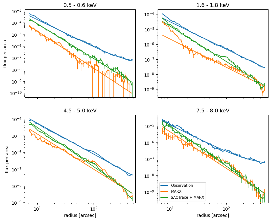
The flux in the scattering halo drops as a powerlaw with increasing distance from the source. In these plots, we should look only at the slope, not the absolute normalization because the total count rate is uncertain in the observation due to the severe pile-up, so the input flux to the simulations might be lower than the true flux.
The plots show the data (with purely statistical uncertainties) and powerlaw fits. Due to the background that is part of the observations but not the simulated data, the powerlaw flattens out for the observed data at high and low energies, where the total count number is low and thus the background more important. We add a constant to the powerlaw model to account for this. SAOTrace simulations produce a fairly smooth powerlaw similar to the observations. The pure marx simulations have much larger deviations due to marx’s simplified mirror model.
'''Analyze and plot results - Plot 2'''
slopes = np.zeros((len(energy_bins) - 1, 3))
for i, e in enumerate(energy_bins[:-1]):
for j, name in enumerate(['obs', 'marx', 'saotrace']):
tab = pycrates.read_file(f'profile_{e:3.1f}_{name}.fits')
r = np.mean(tab.get_column('r').values, axis=1)
r_arcsec = r * 0.492
indfit = r_arcsec > 15.
if name == 'obs':
mymod = const1d + pow1d
const1d.c0.val = tab.get_column('SUR_FLUX').values[-1]
else:
mymod = pow1d
data = Data1D('', r[indfit], tab.get_column('SUR_FLUX').values[indfit],
staterror=tab.get_column('SUR_FLUX_ERR').values[indfit])
gfit = Fit(data, mymod, stat=stat, method=opt)
gfit.fit()
slopes[i, j] = pow1d.gamma.val
fig, ax = plt.subplots()
for i, name in enumerate(['Observation', 'MARX', 'SAOTrace + MARX']):
ax.plot(mid_bins, slopes[:, i], label=name)
ax.legend()
ax.set_xlabel('energy [keV]')
ax.set_ylabel('slope of powerlaw')
ax.set_xlim(0, None)
(0.0, 8.115)
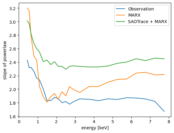
The surface brightness falls off with increasing distance from the source position as a powerlaw. The exponent of this powerlaw depends on the photon energy as shown in the figure. If spectra are extracted in the scattering halo the observed spectrum will thus change with distance from the source. For the observed data, the low energy end (below about 1 keV) has to be taken with a grain of salt. We applied a correction for the ACIS contamination in the data reduction, but the distribution of the contaminant over the detector area is not well known, leading to systematic uncertainties. For energies above 5 keV, the outer mirror shell does not contribute much effective area any longer. This shell has the roughest surface, which explains why we observe steeper powerlaw slopes for higher energies. Both the marx and the SAOTrace mirror model also have energy dependent exponents.
Summary
Both marx and SAOTrace simulations reproduce the wings of the Chandra PSF reasonably well. There are differences in the details, but there is also some uncertainty in the observed data, which, unlike the simulations, contains background events and some detector effects not modeled in marx. It is important to remember though that we study the wings out to several arcminutes here. In all but the brightest sources on the sky, the wings will be undetectable this far out, simply because the total count rate out in the wings is orders of magnitude lower than the in the center of the PSF and will be lost in the background.