Point Spread Function (PSF)
The point-spread function (PSF) for Chandra describes how the light from a point source is spread over a larger area on the detector. Several effects contribute to this, e.g. scatter from not absolutely perfectly shaped mirrors, the uncertainty in the pointing, the fact that the detectors are flat, while the focal plane of the mirror is curved (specifically for large off-axis angles) and the pixalization of data on detector read-out.
The following tests compare marx simulations, SAOTrace simulations, and data to look at different aspects of the Chandra PSF.
On-axis PSF on an ACIS-BI chip
The PSF depends on many things, some of which are common to all observations like the shape of the mirror, and some are due to detector effects. For ACIS detectors, the sub-pixel event repositioning (EDSER) can improve the quality of an image by repositioning events based on the event grade. This correction depends on the type pf chip (FI or BI). This test compares the simulation of a point source on a BI ACIS-S chip to an observation. The observed object is TYC 8241 2652 1, a young star, and was observed in 1/8 sub-array mode to reduce pile-up. The pile-up fraction in the data is about 5% in the brightest pixel.
pars = marxpars_from_asol(asolfile, evt2file)
pars['SpectrumType'] = 'FILE'
pars['SpectrumFile'] = 'input_spec_marx.tbl'
pars['OutputDir'] = 'marx_only'
pars['SourceFlux'] = -1

marxcall = ['marx'] + ['{0}={1}'.format(k, v) for k, v in pars.items()]
marxcall = ' '.join(marxcall)
marxcall

'''Currently, MARX can only be run from the command line. So we build
a command line call from the parameters dictionary and run it via
subprocess.run().'''
out = subprocess.run(marxcall, shell=True, capture_output=True)
# acis_process_events (CIAO 4.18.0): WARNING: The tgain adjustment will not be (re)computed because the doevtgrade is set to no
# acis_process_events (CIAO 4.18.0): WARNING: The values of PHA, ENERGY, PI, FLTGRADE and GRADE may be inaccurate because doevtgrade=no.
# acis_process_events (CIAO 4.18.0): WARNING: The values of ENERGY and PI may be inaccurate because calculate_pi=no.
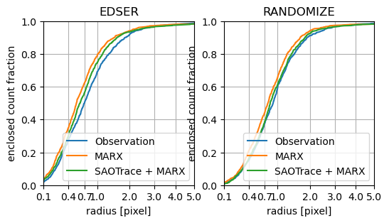
Enclosed count fraction for observation and simulations. The simulations are run with a count number similar to the (fairly short) observation and thus there is some wiggling due to Poisson noise. On the left, the results using the default EDSER algorithms are shown, on the right, the sub-pixel positions are randomized within the pixel independent of the flight grade, which smooths out the inner PSF and hides the problem that marx does not make good predictions for the flight grades.
For BI chips (here ACIS-S3) the marx simulated PSF is too narrow. This effect is most pronounced at small radii around 1 pixel. At larger radii the marx simulation comes closer to the observed distribution. Running the simulation with a combination of SAOTrace and marx gives PSF distributions that are closer to the observed numbers. However, in the range around 1 pix, the simulations are still too wide. Depending on the way sub-pixel information is handled, there is a notable difference in the size of the effect. Using energy-dependent sub-pixel event repositioning (EDSER) requires not only a good mirror model, but also a realistic treatment of the flight grades assigned on the detector. This is where the difference between simulation and observations is largest.
The figures show that there are at least two factors contributing to the difference: The mirror model and problems in the simulation of the EDSER algorithm.
The put those numbers into perspective: If I used the marx simulation to determine the size of the extraction region that encloses 80% of all source counts, I would find a radius close to 0.9 pixel. However, in reality, such a region will only contain about 65% of all flux, causing me to underestimate the total X-ray flux in this source by 15%. (The exact number depends on the spectrum of the source in question.)
On-axis PSF on an ACIS-FI chip
Same as above for a FI chip. The target of this observations is tau Canis Majores.
# acis_process_events (CIAO 4.18.0): WARNING: The tgain adjustment will not be (re)computed because the doevtgrade is set to no
# acis_process_events (CIAO 4.18.0): WARNING: The values of PHA, ENERGY, PI, FLTGRADE and GRADE may be inaccurate because doevtgrade=no.
# acis_process_events (CIAO 4.18.0): WARNING: The values of ENERGY and PI may be inaccurate because calculate_pi=no.
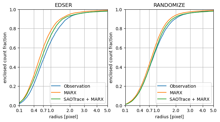
Enclosed count fraction for observation and simulations in the same format as above, but for an ACIS-I observation.
As for the BI chip, marx simulations indicate a PSF that is narrower than the observed distribution. Using SAOTrace as a mirror model, gives better results but still differs significantly from the observed distribution.
On-axis PSF for an HRC-I observation
Same as above for an HRC-I observations of AR Lac.
Since the HRC has no intrinsic energy resolution, the source spectrum can not be taken from the observed data. Instead, we fitted a model to a grating spectrum of the same source and saved that model spectrum to a file. AR Lac is known to be time variable and to show stellar flares, so this spectrum is only an approximation, but it is the best we can do here.
Just as an example, this is the marx call that is used to generate the underlying marx simulation (unfold the boxes with the script code to see more details on how the input parameters are set):
'marx RA_Nom=332.16369387119 Dec_Nom=45.739883051807 Roll_Nom=301.39740584162 GratingType=NONE ExposureTime=18161.46342998743 DitherModel=FILE DitherFile=13182/primary/pcadf13182_000N001_asol1.fits TStart=408913236.56726 SourceRA=332.17 SourceDEC=45.742306 DetectorType=HRC-I DetOffsetX=0.0014262321171452097 DetOffsetZ=-0.0025143152978017724 SpectrumType=FILE SpectrumFile=data/ARLac_input_spec_marx.tbl OutputDir=marx_only SourceFlux=-1'
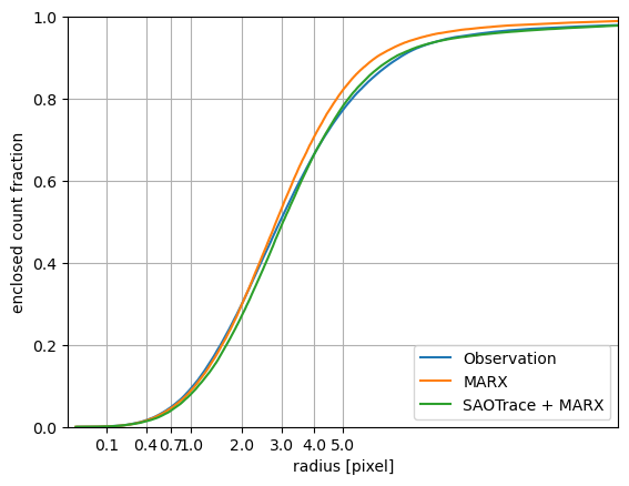
Enclosed count fraction for observation and simulations.
The PSF predicted by SAOTrace + marx tracks the general shape of the observed PSF well, though differences are apparent in the core and in the wings. Like in ACIS, the PSF simulated with marx alone is narrower than the observed PSF.
Off-axis PSF
For an off-axis source the differences between detector pixel size and different event repositioning algorithms is not important. Instead, the size of the PSF is dominated by optics errors because the detector plane deviates from the curved focal plane and because a Wolter type I optic has fundamental limitations for off-axis sources.
The PSF is much larger and no longer circular. As this test shows, the shadows of the support struts become visible.
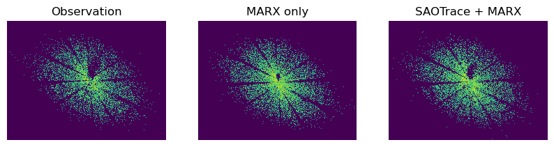
The structure of the PSFs is very similar, emphasizing how good both mirror models are. On closer inspection, there is a small shadow just above and to the right of the point where the support strut shadows meet. This feature is a little smaller in marx than in SAOTrace or the real data due to the simplification that the marx mirror model makes.
On-axis PSF at different energies
The gold standard to test the fidelity of marx and SAOTrace obviously is to compare simulations to observations. However, it is also instructive to look at a few idealized cases with no observational counterpart so we can simulate high fidelity PSFs with a large number of counts without worrying about background or pile-up. The Chandra Proposers Observatory Guide contains a long section on the PSF and encircled energy based on SAOTrace simulations. Some of those simulations are repeated here to compare them to pure marx simulations. For the marx part of the simulation, we assume that both the mirrors reflect every photon and the detectors detect every photon. That way, the simulation gives more photons in the same runtime. That means the |marx|-only simulations will have more photons in the same exposure time than the SAOTrace + |marx| simulations sp the PSF will look a bit more smooth.
for e in energy:
    out = subprocess.run(f'marx SourceType=SAOSAC SAOSACFile="sao{e}.fits" DitherModel=FILE DitherFile="sim_asol.fits" OutputDir="saomarx_{e}" ' +
                     default_marx, shell=True, capture_output=True)
    out2 = subprocess.run(f'marx2fits --pixadj=NONE saomarx_{e} saomarx_{e}.fits',
                          shell=True, capture_output=True)
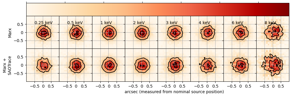
PSF images for different discrete energies for pure marx and SAOTrace + marx simulations. The color scale is linear, but the absolute scaling is different for different images, because the effective area of the mirror and thus the number of detected photons is lower at higher energies. Contour lines mark flux levels at 30%, 60%, and 90% of the peak flux level. At higher energies, the PSF becomes asymmetric, because mirror pair 6, which is most important at high energies, is slightly tilted with respect to the nominal aimpoint. At the same time, the scatter, and thus the size of the PSF, increase at higher energies.
Because the simulations are done with Monte-Carlo methods and the number of photons simulated is finite (but large compared to typical observations), there is some noise in the images.
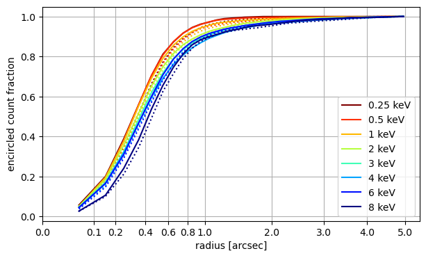
A different way to present the width of the PSF is the encircled count fraction. For each photon, the radial distance is calculated from the nominal source position. Because the center is offset for hard photons, the PSF appears wider at those energies. solid line: marx only, dotted lines: SAOTrace + marx.
marx and SAOTrace simulations predict a very similar PSF shape, but for most energies the SAOTrace model predicts a slightly broader PSF.
Simulated off-axis PSF
Compare marx and SAOTrace + marx simulations for different off-axis angles. For simplicity, this is done here for a single energy. We pick 4 keV because it is roughly the center of the Chandra band.
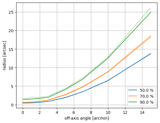
Radius of encircled count fraction for different off-axis angles. The values shown include the effect of the HRC-I positional uncertainty and the uncertainty in the aspect solution. solid line: marx only, dotted lines: SAOTrace + marx
Both simulations show essentially identical off-axis behavior in this test.
